Frequency response is the quantitative measure of the output spectrum of a system or device in response to a stimulus, and is used to characterise the dynamics of the system. It is a measure of magnitude and phase of the output as a function of frequency, in comparison to the input. It is a used to compute structural response when is applied a steady oscillation, like rotating machinery, helicopter blades, etc. Forces can be in the form of applied forces and/or enforced motions (displacements,velocities, or accelerations). In nature the oscillatory loading is sinusoidal.
The steady-state oscillatory response occurs at the same frequency as the loading. The response may be shifted in time due to damping in the system.
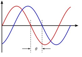
Figure 1: Phase shift.
The important results obtained from a frequency response analysis usually include the displacements, velocities, and accelerations of grid points as well as the forces and stresses of elements. The computed responses are complex numbers defined as magnitude and phase (with respect to the applied force) or as real and imaginary components, which are vector components of the response in the real/imaginary plane. Two different numerical methods can be used in frequency response analysis. The direct method solves the coupled equations of motion in terms of forcing frequency. The modal method utilizes the mode shapes of the structure to reduce and uncouple the equations of motion. The choice of the method depends on the problem.
Direct Frequency Response Analysis
The structural response is computed at discrete excitation frequencies by solving a set of coupled matrix equations. Begin with the damped forced vibration equation of motion with harmonic excitation:
![]()
[B] is the damping matrix, [K] is the stiffness matrix. The load is introduced as a complex vector, the load can be real or imaginary. For harmonic motion (which is the basis of a frequency response analysis), assume a harmonic solution of the form:
{x}={ u (ω) } ei ωt (1)
where { u (ω) } is a complex displacement vector. Taking the first and second derivatives, replacing in the equation and dividing by ei ωt :
[-ω2 M + i ωB + K] { u (ω) } = { P (ω) } (2)
This equation is solved by inserting the forcing frequency, and it represents a system of equations with complex coefficients if dampingis included or the applied loads have phase angles. The equations of motion at each input frequency are then solved in a manner similar to a statics problem using complex arithmetic. Damping simulates the energy dissipation characteristics of a structure. I can be accounted by damping elements CVISC, CDAMPi, and the direct Input Damping Matrixs B2GG and B2PP.
Modal Frequency Response Analysis
This method uses the mode shapes of the structure to reduce the size, uncouple the equations of motion (when modal or no damping is used), and make the numerical solution more efficient. Since the mode shapes are typically computed as part of the characterization of the structure, modal frequency response is a natural extension of a normal modes analysis. As a first step in the formulation, transform the variables from physical coordinates to modal coordinates by assuming:
{x}= [ φ] { ξ (ω) } ei ωt (3)
The mode shapes are used to transform the problem in terms of the behavior of the modes [φ] as opposed to the behavior of the grid points. To proceed, temporarily ignore all damping, which results in the undamped equation for harmonic motion:
-ω2 [M ] {x} + [K ] {x} = { P (ω) } (4)
at forcing frequency ω. Substituting the (3) in (4), dividing by ei ωt and premultiply by to obtain [φT] the following is obtained:
-ω2 [φ ]T [M ] [φ ]{ ξ (ω) } + [φ]T [K] [φ]{ ξ (ω) } = [φ]T { P (ω) }
where:
[φ]T [M ] [φ ] = modal (generalized) mass matrix
[φ ]T [K ] [φ] = modal (generalized) stiffness matrix
[φ]T {P} = modal force vector
The generalized mass and stiffness matrices are diagonal and do not have the off-diagonal terms that couple the equations of motion. Therefore, in this form the modal equations of motion are uncoupled. In this uncoupled form, the equations of motion are written as a set of uncoupled single degree-of-freedom systems as:
-ω2miξi (ω) + Ki ξi (ω) = pi (ω)
where:
mi = i-th modal mass
Ki = i-th modal stiffness
pi = i-th modal force
The modal form of the frequency response equation of motion is much faster to solve than the direct method because it is a series of uncoupled single degree-of-freedom systems. If the damping [B] matrix exists, the orthogonality property of the modes does not, in general, diagonalize the generalized damping matrix and the the generalized stiffness matrix:
[φ ]T [B ] [φ ]≠ diagonal
[φ]T [K ] [φ ]≠ diagonal
In the presence of a matrix [B] or a complex stiffness matrix, the modal frequency approach solves the coupled problem in terms of modal coordinates using the direct frequency approach. When modal damping is used, each mode has damping bi where bi = 2mi ωiξi. The equations of motion remain uncoupled and have the form for each mode:
-ω2miξi (ω) + i ωbiξi (ω) + Ki ξi (ω) = pi (ω)
And the model response is computed using:
ξi (ω) = pi (ω) / (-ω2mi + i ωbi+ Ki)
The TABDMP1 Bulk Data entry defines the modal damping ratios, where the frequency/damping pairs are specified, the damping value has to be applied to specific value of the frequency. The TABDMP1 table is activated by selecting the Table ID with the SDAMPING Case Control command.
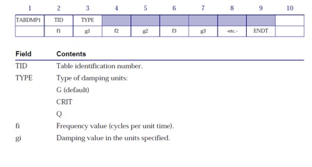
Figure 2 – TABDMP1 entry Nastran
The three type of damping are related to the following equations:
– ξi = bi / bcr = Gi / 2 – structural damping (default)
– bcr = 2 mi ω – critical damping
– Q = 1 / (2 ξi) = 1 / Gi – quality factor
the subscript is for the i-th mode
For theoretical description of the damping ratio click here
Linear interpolation is used for modal frequencies between consecutive values. ENDT ends the table input. Below there is an exemple of the interpolation / extrapolation for the modal damping. The frequency of 1 Hz is extrapolated by the entries at f = 2.0 and 3.0 Hz.
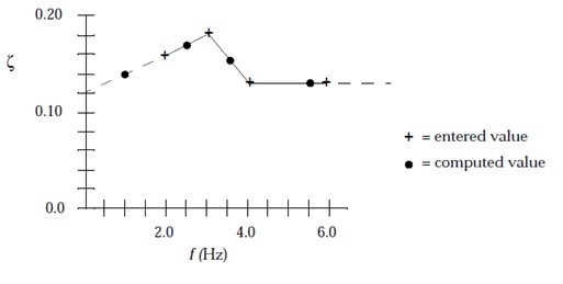
Figure 3: TABDMP1
|
Entered |
Computed |
||
|
f (Hz) |
z |
f (Hz) |
z |
|
2.0 |
0.16 |
1.0 |
0.14 |
|
3.0 |
0.18 |
2.5 |
0.17 |
|
4.0 |
0.13 |
3.6 |
0.15 |
|
6.0 |
0.13 |
5.5 |
0.13 |
Table 1: Example TABDMP1 Interpolation/Extrapolation
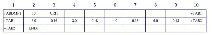
Figure 4: TABDMP1 entry
The decoupled solution procedure used in modal frequency response can be used only if either no damping is present or modal damping alone (via TABDMP1) is used. Otherwise, the modal method uses the coupled solution method on the smaller modal coordinate matrices if nonmodal damping (i.e., CVISC, CDAMPi, GE on the MATi entry, or PARAM,G) is present. The modes whose resonant frequencies lie within the range of forcing frequencies must to be retain. For example, if the frequency response analysis must be between 100 and 3000 Hz, all modes whose resonant frequencies are in this range should be retained. For better accuracy, all modes up to at least two to three times the highest forcing frequency should be retained.
We can select a specific range of mode frequencies by the eigenvalue entry (EIGRL or EIGR). Since for the default all computed modes are retained, three parameters are available to limit the number of modes included in the solution. PARAM,LFREQ gives the lower limit on the frequency range of retained modes, PARAM,HFREQ gives the upper limit, PARAM,LMODES gives the number of lowest modes to be retained. In modal frequency response analysis, two options are available for recovering displacements and stresses: the mode displacement method and the matrix method. Since the number of modes is usually much less that the number of excitation frequencies, the matrix method is usually more efficient and is the default. The mode displacement method can be selected by using PARAM,DDRMM,-1 in the Bulk Data.
Modal Versus Direct Frequency Response
In general, larger models may be solved more efficiently in modal frequency response because the numerical solution is a solution of a smaller system of uncoupled equations. The major portion of the effort in a modal frequency response analysis is the calculation of the modes. For large systems with a large number of modes, this operation can be as costly as a direct solution. The direct method is more accurate than the modal method because the direct method is not concerned with mode truncation.
|
|
Modal |
Direct |
|
Small Model |
|
● |
|
Large Model |
● |
|
|
Few Excitation Frequencies |
|
● |
|
Many Excitation Frequencies |
● |
|
|
High Frequency Excitation |
|
● |
|
Nonmodal Damping |
|
● |
|
Higher Accuracy |
|
● |
Table 2: Modal versus Direct Frequency response
Excitation Definition
In a frequency response analysis, the force must be defined as a function of frequency. Forces are defined in the same manner for the direct and modal method. The following Bulk Data entries are used for the frequency-dependent load definition:
RLOAD1 – Tabular input-real and imaginary
RLOAD2 – Tabular input-magnitude and phase
DAREA- Spatial distribution of dynamic load
LSEQ – Generates the spatial distribution of dynamic loads from static load entries
DLOAD – Combines dynamic load sets
TABLEDi – Tabular values versus frequency
DELAY – Time delay
DPHASE – Phase lead
Only concentrated forces and moments can be specified directly using DAREA entries. To accommodate more complicated loadings conveniently, the LSEQ entry is used to define static load entries that define the spatial distribution of dynamic loads. The frequency variation in the loading is the characteristic that differentiates a dynamic load from a static load (temporal distribution of the load)
– Frequency-Dependent Loads – RLOAD1 Entry
It defines a dynamic loading of the form:
{P (f)} = { A[C( f ) + i D( f )] ei{θ-2π fτ}
The values of the coefficients are defined in tabular format on a TABLEDi entry. You need not explicitly define a force at every excitation frequency. Only those values that describe the character of the loading are required. MSC.Nastran will interpolate for intermediate values.
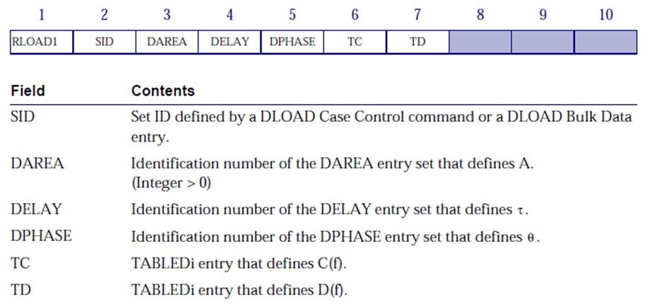
Figure 5: RLOAD1 Entry
– Frequency-Dependent Loads – RLOAD2 Entry
The RLOAD2 entry is a variation of the RLOAD1, which defines the real and imaginary parts of the complex load, instead the RLOAD2 entry defines the magnitude and phase.
{P (f)} = { AB( f ) ei{Φ(f) + θ – 2π fτ} }
RLOAD1 = RLOAD2
C( f ) + i D( f ) = B( f ) eiΦ(f)
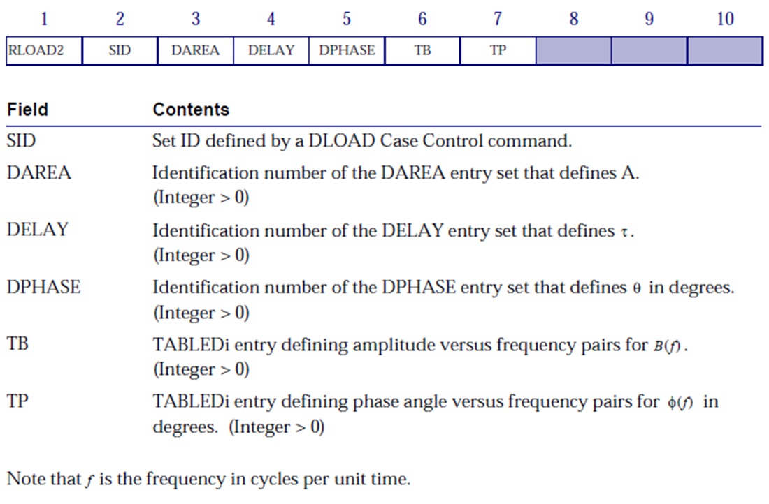
Figure 6: RLOAD2 Entry
– Spatial Distribution of Loading — DAREA Entry
The DAREA entry defines the degrees-of-freedom where the dynamic load is to be applied and the scale factor to be applied to the loading.
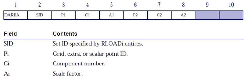
Figure 7: DAREA Entry
A DAREA entry is selected by RLOAD1 or RLOAD2 entries, and several of DAREA entries may be used. The DELAY entry defines the time delay in an applied load and the DPHASE entry defines the phase lead, either must to be defined with same grid point and component (see the Nastran quick guide for further informations).
– Dynamic Load Tabular Function – TABLEDi Entries
The TABLEDi entries (i = 1 through 4) each define a tabular function for use in generating frequency-dependent dynamic loads. The form of each TABLEDi entry varies slightly, depending on the value of i, as does the algorithm for y(x). The x values need not be evenly spaced. The TABLED1, TABLED2, and TABLED3 entries linearly interpolate between the end points and linearly extrapolate outside of the endpoints, as shown in the figure below.
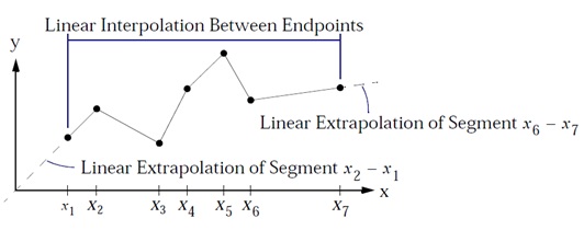
Figure 8: Interpolation and Extrapolation for TABLEDi Entries
The TABLED1 entry uses the algorithm:
y = yT(x )
See the Nastran Quick Reference for the TABLED2, and TABLED3. The choise of the TABLEDi depends of which algorithms is necessary for the interpolation and extrapolation of x and y entries.
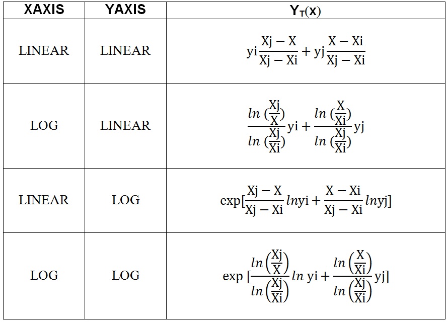
Table 2: algorithms used for interpolation and extrapolation
– Static Load Sets – LSEQ Entry
Since concentrated forces and moments can be specified directly using DAREA entries, to permit more flexibility and to use more complicated loadings the LSEQ entry is used. By this entry the DAREA has to be referred but without to use it, it is enough to use the same ID related to DAREA in RLOAD1 and LSEQ cards. By the commands in the Case Control Section shown below, In figure 4 is clear its use.
LOADSET = 27
DLOAD = 25
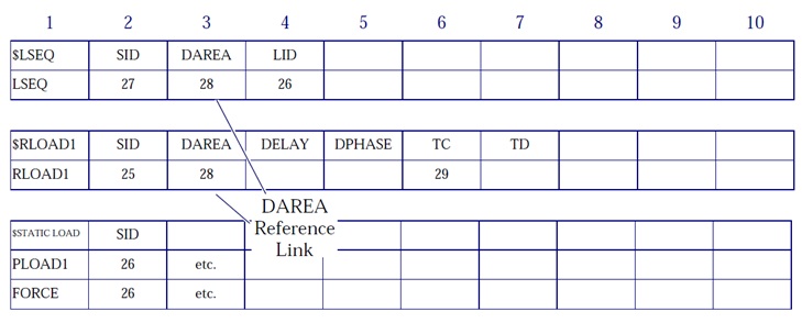
Figure 10: DAREA Reference Link
The Load Set ID may refer to one or more static load entries (FORCE, PLOADi, GRAV, etc.).
– Dynamic Load Set Combination – DLOAD
The total applied load is constructed from a linear combination of component load sets as follows:
{P}= S ∑iSi{Pi}
S is the overall scale factor, Si scale factor for the i-th load set, Pi i-th load set. DLOAD Bulk Data entry has the following format:
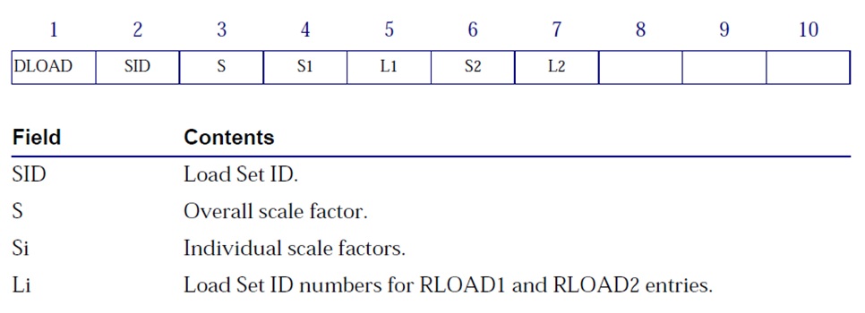
Figure 11: DLOAD Entry
Excitation frequency
There are six Bulk Data entries that you can use to select the frequency at which the solution is to be performed. Each specified frequency results in an independent solution at the specified excitation frequency.
FREQ – Defines descrete excitation frequencies and entry specifies ten specific loading frequencies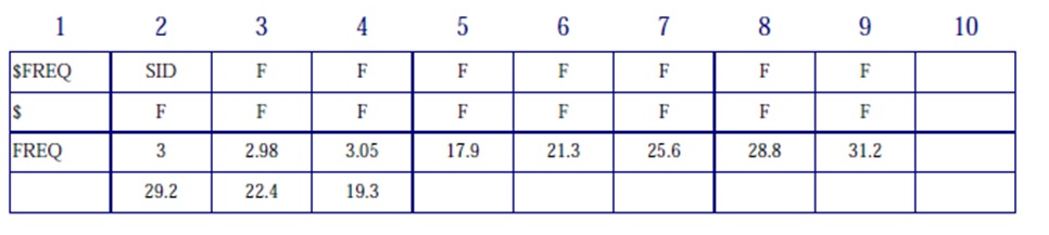
FREQ1 – Defines a starting frequency Fstart, a frequency incitement ∆f, and the number of frequency increments to solve NDF.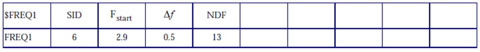
FREQ2 – Defines a starting frequency Fstart, and ending frequency Fend, and a number of logaritmic intervals NF, to be used in the frequency range.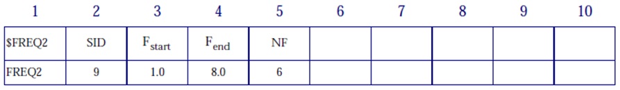
FREQ3 – Used for modal solution only, it defines the number of excitation frequencies (NEF) used between modal pairs (F1, F2) in a given range. By TYPE field is possible use linear (LINEAR, Default) or logarithmic (LOG) interpolation between frequencies. By a CLUSTER value greater than 1 provides closer spacing of excitation frequencies near the modal frequencies, where greater resolution is needed. 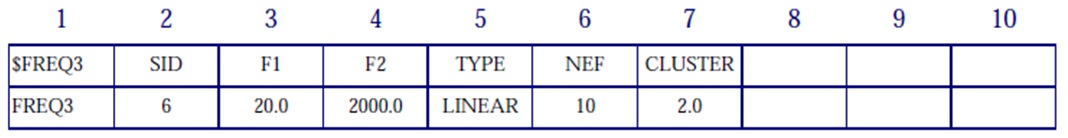
FREQ4 – Used for modal solution only, it defines excitation frequencies using a spread about each normal mode within a range. F1 and F2 are respectively lower and upper bound of modal frequency range. The example FREQ4 chooses 21 equally spaced frequencies across a frequency band of 0.7 fN to 1.3 fN for each natural frequency between 20 and 2000. 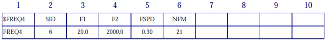
FREQ5 – Used for modal solution only, it defines excitation frequencies as all frequencies in a given range (F1 and F2 are respectively lower and upper bound of modal frequency range) as a defined fraction (FRi) of the normal modes.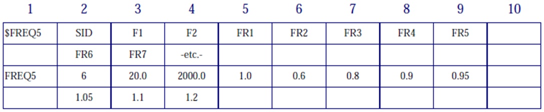
Considerations
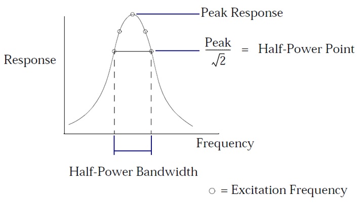
Undamped or very lightly damped structures exhibit large dynamic responses for excitation frequencies near resonant frequencies. Use a fine enough frequency step size (∆f ) to adequately predict peak response. Use at least five points across the half-power bandwidth (which is approximately 2ξfn for an SDOF system) as shown in the Figure below.
For maximum efficiency smaller frequency spacing should be used in regions near resonant frequencies, and larger frequency step sizes should be used in regions away from resonant frequencies.
Examples
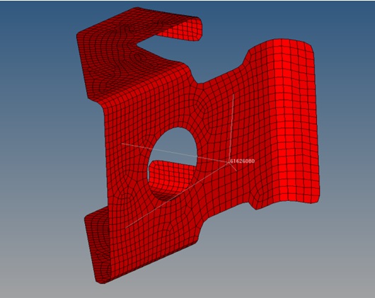
1) Bracket
Consider the bracket model shown in Figure below. An oscillating gravity load of 9*g = 9*9.81m/s2 =88.29 m/s2 is applied to the entire item in the z-direction. The model is constrained at its base. Modal frequency response is run from 0 to 140 Hz with a frequency step size of 0.2 Hz. Eigenvalues to 1000 Hz are computed using the Lanczos method. No modal damping is applied.
Below is shown the input BDF file. The LSEQ entry is used to apply the gravity loads (GRAV entries). Note that the LSEQ and RLOAD1 entries reference a common DAREA ID (the node 61626080) and that there is no explicit DAREA entry.
$ NASTRAN input file
SOL 111
TIME 400
$ Direct Text Input for Executive Control
CEND
TITLE = BRK MODEL
SUBTITLE = MODAL FREQUENCY RESPONSE ANALYSIS
ECHO = NONE
$
$ SPECIFY SPC
SPC = 3
$
$ SPECIFY MODAL EXTRACTION
METHOD = 777
$
$ SPECIFY DYNAMIC INPUT
DLOAD = 2
$ SDAMPING = 4
LOADSET = 3
FREQUENCY = 5
$ OUTPUT REQUEST
$ Frequencies for which output will be printed in frequency response
SET 123 = 61626080
DISPLACEMENT(PHASE,PLOT)=123
$
$ XYPLOTS
$
$… X-Y plot commands …
$
OUTPUT(XYPLOT)
$ XTGRID: Controls the drawing of the grid lines parallel to the x-axis at the y-axis tic marks on upper half frame
$ curves only.
XTGRID = YES
YTGRID = YES
$ XBGRID: Controls the drawing of the grid lines parallel to the x-axis at the y-axis tic marks on lower half frame
$ curves only.
XBGRID = YES
YBGRID = YES
$
$ PLOT RESULTS
XTITLE = FREQUENCY
$
$ YTLOG: Selects logarithmic or linear y-axis for upper half frame curves only. YES – > Plot a logarithmic y-axis. NO Plot a linear y-axis
$ T2RM, Ti stands for the i-th translational component, RM means real or magnitude, IP means imaginary or phase
YTTITLE = DISPL. MAG. 61626080
YBTITLE = DISPL. PHASE 61626080
XYPLOT,XYPUNCH,DISP /61626080(T3RM,T3IP)
YTTITLE = DISPL. MAG. 61626080
YBTITLE = DISPL. PHASE 61626080
XYPLOT,XYPUNCH,DISP /61626080(R3RM,R3IP)
$
BEGIN BULK
$
$…….2…….3…….4…….5…….6…….7…….8…….9…….10…..$
$
$ NORMAL MODES TO 200 HZ
$EIGRL SID V1 V2
EIGRL 777 -0.1 1000.
$ EXCITATION FREQUENCY DEFINITION 0 TO 140 HZ
$FREQ1 SID F1 DF NDF
FREQ1 5 0.0 0.2 800
$ DYNAMIC LOADING
$RLOAD1 SID DAREA DELAY DPHASE TB TP
RLOAD1 2 61626080 22
$
$LSEQ SID DAREA LID TID
LSEQ 3 61626080 1
$TABLED1 TID
$+TABL1 X1 Y1 X2 Y2 ETC.
TABLED1 22
0.0 1.0 1000.0 1.0 ENDT
$$$ LOAD $$$
$ Gravity Loading of Load Set : DWD with gz, 9810*-9=-88290
GRAV 1 0 -88290. 0. 0. 1.
$ Direct Text Input for Bulk Data
include ‘Bulk_DFEM.bdf’
ENDDATA
The Figure below shows a logarithmic plot of the z-displacement and rotation magnitude of grid point 61626080, which is the concentrated mass at the center of the cutout.
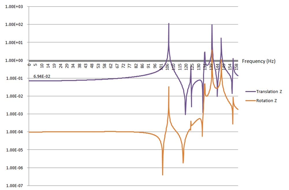
Logarithmic plots are especially useful for displaying frequency response results since there can be several orders of magnitude between the maximum and minimum response values. The output is generated by OUTPUT(XYPLOT) card. In output a .plt file and .pch files are generated. If you don’t have the NASTRAN NASTPLT Post Processor, you can produce the plot by mean the pch file, importing it in excel and creating easly the curves shown above. Where the current frequency corresponds to the modal frequency (in this case for the first mode is 107 Hz) for the resonance reason, the displacement is much higher (mainly for the displacement, since the load is not a rotation), there is a singularity.
2) Beam Model
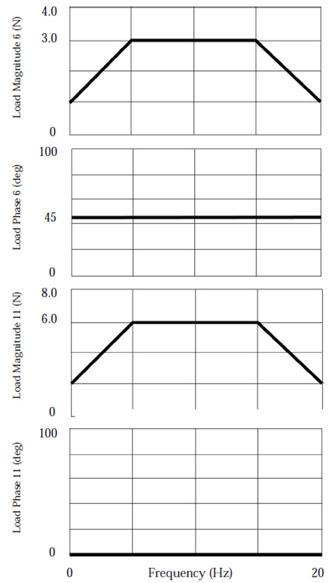
Consider a unidimensional model of the cantilever beam shown in the Figure below with unrestrained DOFs in the T2 and R3 directions. Two loads are applied: one at grid point 6 and the other at grid point 11. The loads have the frequency variation shown in Figure below. The loads in the figure are indicated with a heavy line in order to emphasize their values. The load at grid point 6 has a 45-degree phase lead, and the load at grid point 11 is scaled to be twice that of the load at grid point 6. Modal frequency response is run across a frequency range of 0 to 20 Hz. Modal damping is used with 2% critical damping between 0 and 10 Hz and 5% critical damping above 10 Hz. Modes to 500 Hz are computed using the Lanczos method.

Below it is listed the input file:
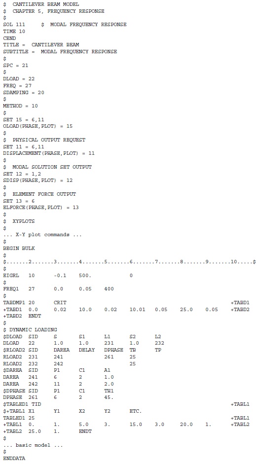
Note that the DLOAD Bulk Data entry references two RLOAD2 entries, each of which references a separate DAREA entry and a common TABLED1 entry. The RLOAD2 entry for grid point 6 also references a DPHASE entry that defines the 45-degree phase lead. The RLOAD2 entry describes a sinusoidal load in the form:
{P (f)} = { AB( f ) ei{Φ(f) + θ – 2π fτ} }
where:
A = 1.0 for grid point 6 and 2.0 for grid point 11 (entered on the DAREA entry)
B = function defined on the TABLED1 entry
Φ = 0.0 (field 7 of the RLOAD2 entry is blank)
Θ = phase lead of 45 degrees for grid point 6 (entered on the DPHASE entry)
τ = 0.0 (field 4 of the RLOAD2 entry is blank)
Logarithmic plots of the output are shown in the following figures. Figure 11 shows the magnitude of the displacements for grid points 6 and 11. Figure 12 shows the magnitude of the modal displacements for modes 1 and 2. Figure 13 shows the magnitude of the bending moment at end A in plane 1 for element 6.
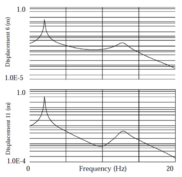
Figure 11: Displacement Magnitude (Log)
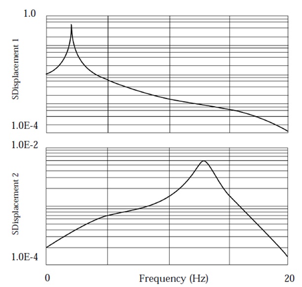
Figure 12: Modal Displacement Magnitude (Log)
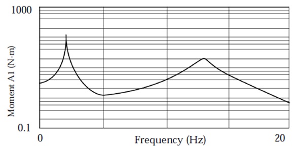
Figure 12: Bending Moment Magnitude at End A, Plane 1 (Log)
Download the original file: FrequencyResponse.zip
3 Responses to Frequency Response – Nastran SOL 111