In the most of cases the nonlinear effects in structures occur due to nonlinear material behavior and large deformations. Geometric nonlinearity becomes relevant when the structure is subjected to large displacement and rotation. Geometric nonlinearity effects are prominent in two aspects: geometric stiffening due to initial displacements and stresses, and follower forces due to a change in loads as a function of displacements. Material nonlinear effects may be classified into many categories. They are plasticity, nonlinear elasticity, creep, visco elasticity. The solution 106 uses an iterative process based on the modified Newton’s method.
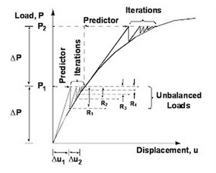
The primary solution operations are gradual load or time increments (as shown by DP in Figure 1), iterations with convergence tests for acceptable equilibrium error (indicated by R1, R2 …) and stiffness matrix updates. The iterative process is based on the modified Newton’s method. The stiffness matrix is updated as per the selection of the iterative method (which has effect on computational efficiency).
General Solution Structure:
SOL 106
CEND
TITLE = TEST
DISP = ALL
STRESS = ALL
SPC = 1
SUBCASE 1
SUBTITLE = ELASTIC — Load at 85%
LABEL = Load in Elastic Field
LOAD = 50
NLPARM = 50
SUBCASE 2
SUBTITLE = PLASTIC — Load at 100%
LABEL = Load in Plastic Fielad, the Yield limit is passed
LOAD = 100
NLPARM = 100
$ END OF CASE CONTROL DATA
$ BULK DATA SECTION
BEGIN BULK
NLPARM 50 1 AUTO UPW NO
NLPARM 100 8 SEMI UPW NO
….
….
….
ENDDATA
General Recommendation:
– A simple model to understand the behavior of the structure is advisable.
– The model has to be a compromise between the accuracy and the efficency of the analysis
– A finer mesh is advisable in the area of interest
– Avoid stiff elements like TRIA3 and TET4, the solution convergence could be more difficult
Nonlinear static analysis permits only one independent loading condition per run, while in a linear analysis subcases represent an independent loading condition and each subcase is distinct from all others. A non linear analysis is path dependent , the loads and position are incremented step by step, the changes are in the subcase are cumulative. The NLPARAM is the parameter which controls the non linear analysis, it defines strategies for the incremental and iterative solution processes. It is difficult to choose the optimal combination of all the options for a specific problem. The default option was intended to provide the best workable method for a general class of problems, users should start with the default option. When by default parameters the convergence is not reached, by some changes it is possible to get the solution.
NLPARM Card
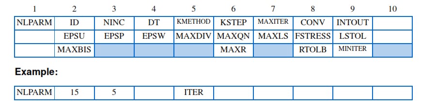
The NLPARM entry controls the incremental and iterative solution processes. It defines strategies for the incremental and iterative solution processes. It is difficult to choose the optimal combination of all the options for a specific problem. However the default option was intended to provide the best achievable method for a general class of problems.
1) The NINC field is an integer which specifies the number of increments to be processed in the subcase. The total load specified in the subcase minus the load specified in the preceding subcase is equally divided by this integer (NINC) to obtain the incremental load for the current subcase. Another subcase should be defined to change constraints or loading paths. However, multiple subcases may be required in the absence of any changes in constraints or loads to use a moderate value (e.g., not to exceed 20) for NINC. Use of a moderate value has advantages in controlling database size, output size, and restarts.
2) The strategies to update the Stiffness matrix are determined by a combination of the data specified in the two fields KMETHOD and KSTEP. Options for KMETHOD are AUTO, SEMI, or ITER. The KSTEP field, which is an auxiliary to the KMETHOD field, should have an integer equal to or greater than 1.
1) The MAXITER field is an integer representing the number of iterations allowed for each load increment. If the number of iterations reaches MAXITER without convergence, the load increment is bisected and the analysis is repeated. If the load increment cannot be bisected (i.e., MAXBIS is reached or MAXBIS = 0) and MAXDIV is positive, the best attainable solution is computed and the analysis is continued to the next load increment. If MAXDIV is negative, the analysis is terminated. MAXDIVis the limit on probable divergence conditions per iteration before the solution is assumed to diverge, it is based on a energy rate error by means an iteration is defined as diverged.
2) The convergence test is performed at every iteration with the criteria specified in the CONV field. Any combination of U (for displacement), P (for load), and W (for work) may be specified. All the specified criteria must be satisfied to achieve convergence.
3) INTOUT controls the output requests for displacements, element forces and stresses, etc. YES: Gives all outputs at every increment No: Gives output at last increment or load step. It is advisable to use YES to now the status step by step. It is useful to get results with all the steps used for the load increments.
4) The convergence tolerances are specified in the fields EPSU, EPSP, and EPSW for U, P, and W criteria, respectively.
Nonlinear Iteration Method.
– The AUTO method works very well as a starting point and is the default method in the nonlinear static solution. This method essentially examines the solution convergence rate and uses the quasi-Newton, line search and/or bisection methods to perform the solution as efficiently as possible sometimes without a stiffness matrix update. Highly nonlinear behavior in some cases may not be handled effectively using the AUTO method.
– The SEMI method is also an efficient technique for nonlinear static iteration. It is similar to the AUTO method since it uses the quasi-Newton, line search and/or bisection methods, but it differs from the AUTO method in one respect. The SEMI method forces a stiffness matrix update after the first iteration of a load increment. This update is performed irrespective of the convergence status of the solution. It is effective in many highly nonlinear problems where regular stiffness matrix updates help the solution to converge.
– The ITER method is known as the “brute force” method in nonlinear static analysis because a stiffness matrix update is forced at every KSTEPth iterations with a resultant increase in CPU time. Its best applications tend to be those involving highly nonlinear behavior for which using only multiple iterations may not be efficient.
MAXBIS and Convergence Criteria
The incremental load value is bisected automatically if the convergence is not achieved in any incremental load step even after maximum number of iteration defined by the user. Bisection means cutting the time step size or load increment size by half. This bisection occurs mainly due to any large nonlinearity in the model or when the NINC or load increment for the particular load step is too large. Divergence processing uses a combination of stiffness updates and bisections to facilitate convergence. Note: MAXBIS is not written out directly from Patran. It has to be manually included if the default values need to be overwritten
Convergence criterion may be any combination of out-of-balance forces, change in displacements, and energy (work) error. Convergence criterion based on out-of balance force and change in displacement is used before yielding and convergence criterion based on out-of-balance force is used after yielding because displacement is very high after yielding. If a solution for particular load increment (or time step) cannot converge within MAXITER number of iterations, that increment is halved. Solution is attempted again, and if it does not converge again, another halving (bisection in NASTRAN speak) is done, up to a maximum number of bisections controlled by MAXBIS entry on NLPARM entry. Default is 5, max value is 10, but if you have to go higher, it most likely indicates either some irregularity with the model, or that NASTRAN is not the best tool for problem at hand.
1) cNINC from default 10 to 15 or 20
2) Increase MAXBIS, up to 10
3) Change KMETHOD to ITER or SEMI and set KSTEP to 1 (caution: this will slow down the solution significantly, sometimes it is better to use the default value)
4) Increase the values of EUI, EPI, EWI to reach the convergence
Exemple:
NLPARM 1 20 AUTO 5 30 P YES +
+ 0.01
To make that the solution is more fast, put this in the prameter section:
PARAM FOLLOWK NO (requests that the follower force stiffness will not be considered)
Material and Geometric Nonlinearities
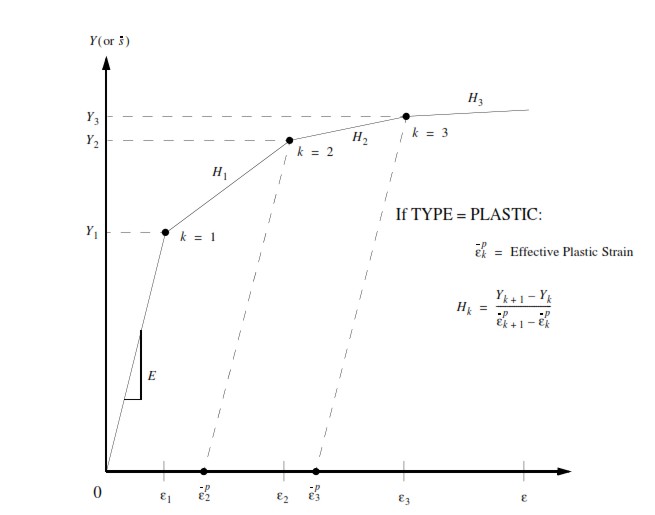
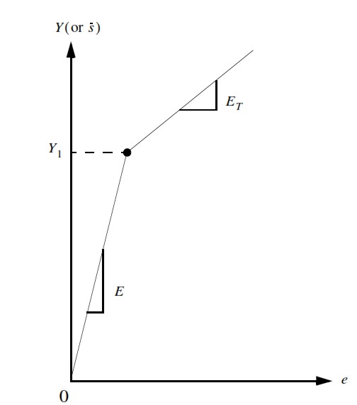
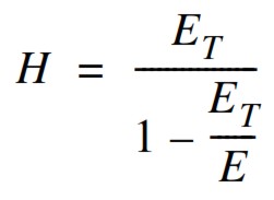
Material Definition – MATS1 and TABLES1. To introduce the material nonlinearity 2 ways are generally adopted, by H parameter or MATS1 + TABLES. Elastoplastic material consists of elastic and a plastic portion in stress-strain curve. The elastic portion is defined by providing the Young’s Modulus, E and Poisson’s ratio, n (MAT1); and the plastic portion is defined using a stress-strain curve data points through tabular input (MATS1 + TABLES1 or ‘FIELDS’ in Patran). A couple of important points to consider while defining stress-strain curve is that the first point must be at the origin (X1 = 0, Y1 = 0) and the second point (X2, Y2) must be at the initial yield point specified on the MATS1 entry. The slope of the line joining the origin to the yield stress must be equal to the value of E. Sometimes when the Stress-Strain curve is not available, is convenient to use the “Hardening slope” H parameter.
LGDlSP = 1, all the nonlinear element types that have a large displacement capability in SOLs 106, 129, 153, 159, 400, and 600 will be assumed to have large displacement effects(updated element coordinates and follower forces).
FOLLOWK=NO requests that the follower force stiffness not be included.
Postprocessing / Output in Nonlinear Static Analysis:
There are two output blocks in SOL 106:
1) Nonlinear stress/strain (for non linear element only)
This is printed as “NONLI EAR STRESSES IN TETRAHEDRON SOLID ELEMENT S (TETRA)” in the *.f06 and it is given by default case control command NLSTRESS = ALL. The Patran stress output label NONLINEAR comes from this table. This is the “True stress.” (This table also contains strains, the strains labeled NONLINEAR come from this output.) The nonlinear stress data is output in the element coordinate system.
2) Linear stress/strain (for linear and nonlinear elements) This is printed as “STRESSES IN TETRAHEDRON SOLID ELEMENTS (CTETRA)” in the *.f06 and it is given by default case control command STRESS = ALL. In Patran it is shown as “STRESS TENSOR”. In short it is the “equivalent linear stress”. You can also ask for STRAIN=ALL, this is the STRAIN TENSOR.
The stresses at center should match in both cases, however due to extrapolation, linear and nonlinear may not match. Many times the discrepancy is also caused by averaging stresses at node (in fringe plot)
And sometimes if you don’t have perfect elastic plastic the stresses could be higher than yield point as well. You can have a look at the “nonlinear stresses, stress tensor” with the centroidal values. It will give you the best correlation with hand calculations. [Nonlinear stresses are given for nodal as well as centroid]
Nastran nonlinear stress request (NLSTRESS) contains both – stress and strain. Whereas for linear elements (e.g.: CBAR), one has to request stress and strain separately (STRESS=ALL/STRAIN=ALL)
“STRESS TENSOR” is applicable for all the elements – (linear and nonlinear elements)
“NONLINEAR STRESSES, STRESS TENSOR” is applicable for nonlinear elements ONLY (e.g.: BEAM, TETRA (4&10)). “NONLINEAR STRESSES, EQUIVALENT STRESSES” is applicable to Von-Mises stresses in Non-Linear elements
“The results that you see marked as “Stress Tensor” in Patran from your nonlinear run are linear stresses based on nonlinear displacements, and the results marked as “Nonlinear Stresses, Stress Tensor” are the true nonlinear stresses. The ones marked “Nonlinear Stresses, Equivalent Stress” are a Von Mises stress calculation.”
“STRAIN TENSOR” is same as stress tensor, but Strain Values – (for both linear and nonlinear elements). PLASTIC STRAIN is strain beyond the elastic limit.
When post-processing strain results in PATRAN, the results menu under “create Fringe plot” allows for two strain values the user can plot:
A) Nonlinear strains, plastic strain; and
B) Nonlinear strains, strain tensor
Choice “A” is consistent with the value from the .f06 file under the EFF. STRAIN/ PLAS/NLELAS column from the NLSTRESS case control request.
Choice “B” is consistent with the value from the .F06 file under STRAIN output you got from STRAIN=ALL case control command.
“The results that you see marked as “Stress Tensor” in Patran from your nonlinear run are linear stresses based on nonlinear displacements, and the results marked as “Nonlinear Stresses, Stress Tensor” are the true nonlinear stresses. The ones marked “Nonlinear Stresses, Equivalent Stress” are a Von Mises stress calculation.”
How to understand convergence, output in F06:
EUI: Normalized error in the displacement.
EPI: Normalized error in the load vector.
EWI: Normalized error in the energy.
LAMBDA: Rate of convergence. Solution is diverging if it is > 1.0.
DLMAG: Absolute norm of the load error vector.
FACTOR: Scale factor for line search method.
E-First: Initial error before line search begins.
E-FINAL: Final error after line search terminates.
N-QNV: Number of quasi-Newton correction vectors to be used in the current iteration.
N-LS: Number of line searches performed.
ENIC: Expected number of iterations for convergence.
NDV: Number of occurrences of probable divergence during the iteration.
MDV: Number of occurrences of bisection conditions due to excessive increments in stress and rotations.
Restriction and Limitations in SOL 106:
- CROD, CBEAM, CGAP, CQUAD4, CQUAD8, CTRIA3, CTRIA6, CHEXA, and CTETRA elements may be defined with material or geometric nonlinear properties. All other elements will be treated as having small displacements and linear materials.
- Constraints apply only to the nonrotated displacements at a grid point. In particular, multipoint constraints and rigid elements may cause problems if the connected grid points undergo large motions. However, also note that replacement of the constraints with overly stiff elements can result in convergence problems.
- Large deformations of the elements may cause nonequilibrium loading effects. The elements are assumed to have constant length, area, and volume, except for hyperelastic elements.
- Since the solution to a particular load involves a nonlinear search procedure, solution is not guaranteed. Care must be used in selecting the search procedures on the NLPARM data. Nearly all iteration control restrictions may be overridden by the user.
- Follower force effects are calculated for loads which change direction with grid point motion.
- Every subcase must define a new total load or enforced boundary displacement. It is necessary because error ratios are measured with respect to the load change.
Common Errors:
Some of the common errors that can be avoided are:
- Slope of elastic curve in MATS1/TABLES1 & Young’s Modulus, E in MAT1 should be same
- Avoid having large load steps. E.g.: If the total load to be applied is say 10000N, break it into 2 or preferably 3 subcases/loadsteps
- In case that the analysis doesn’t reach the convergence, sometimes could be due to an error in the loads applied. For example, in case of pressure applied, if it is wrong, too much high in some zone, the problem is unrealistically too non linear.
- Since the units of convergence tolerance is independent of units, avoid tightening or loosening the tolerance in the first run
- Make sure enough system resources (Memory and Hard Disk Space) are available at hand for large models
- “User Fatal Message 4676 (NMEPD) – ERROR EXCEEDS 20.00 PERCENT OF YIELD STRESS IN ELEMENT ID=XX” may be encountered if there exists large deformation of the nodes of an element or presence of severely distorted elements. In case of large deformation (caused due to extremely large loads), then it is basically a large strain problem (as opposed to small strain assumption in Nastran) which needs to be solved by another solution sequence like MSC Marc or SOL 600. In case of severely distorted element, it is advisable to inspect the element quality in the mesh of the model.
- “USER FATAL MESSAGE 1221 (GALLOC) – THE PARTITION OF THE SCRATCH DBSET USED FOR DMAP-SCRATCH DATABLOCKS IS FULL”. This fatal message is commonly encountered due to low system resources. Note that this fatal will stop writing the results into xdb/op2 completely and no output will be obtained. To avoid this fatal message, include “NASTRAN SYSTEM(151)=1” and increase the buff size “NASTRAN BUFFSIZE=65537” in the NASTRAN SYSTEM CELL SECTION of input file (above Executive Control Section)
- When you use for the material the Hardening method, if you get this error: *** USER FATAL MESSAGE 5423 (SADD5) ATTEMPT TO ADD INCOMPATIBLE MATRICES, it means that the H is too small.
Some further hint to reach Convergence:
- – Increase the tollerance error by increasing EUI, EPI, and EWI paramenters.
- – Try by setting LANGLE=2. LANGLE specifies the method for processing large rotations in nonlinear analysis. By default, large
rotations are computed with the gimbal angle method in nonlinear analyses. If PARAM,LANGLE,2 is specified, then they are
computed with the Rotation Vector method. With this method the convergence is more probable, even if the calculation is slower.
- – Try by setting K6ROT=1000 (Default = 100). K6ROT specifies the scaling factor of the penalty stiffness to be added to the normal rotation for
CQUAD4 and CTRIA3 elements. The normal rotation has no physical meaning and should be ignored. The penalty stiffness removes the singularity in the normal rotation. A higher value than K6ROT=100. is not recommended because unwanted stiffening effects may occur, but somethimes could be useful strategy to undestand if the non-convergence is due to singularity in the normal rotation.