Introduction
Random vibration is motion which is non-deterministic, meaning that future behavior cannot be precisely predicted, and it is a characteristic of the input or excitation. To specific a random vibration is usually is used the ASD (acceleration spectral density). The root mean square acceleration (Grms) is the square root of the area under the ASD curve in the frequency domain, and it express the overall energy of the random vibration.
A PSD curve provides the power of a signal as a function of frequency. For random vibration analysis usually it uses the units of G2/ Hz, G denotes the g-force.
For random vibration, the specification curve is actually an acceleration spectral density (ASD) but is also displayed in “power” terms or measurement units squared as a function of frequency. It’s just a convenient way to express the profile of a random vibration spectra.
While the term power spectral density (PSD) is commonly used to specify a random vibration event, ASD is more appropriate when acceleration is being measured and used in structural analysis and testing.
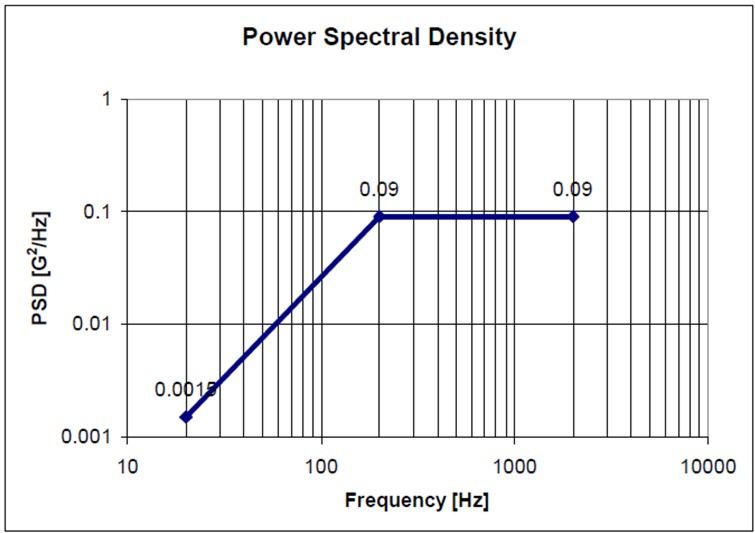
Figure 1: Acceleration Power Spectral Density
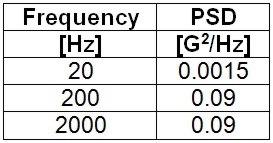
Table 1: Acceleration Power Spectral Density
For the exemple shown above the Grms of the input PSD is 13. This can be calculated by taking the square root of the area under the acceleration spectral density curve. The RMS or Grms value of random vibration spectra is important since it provides a representation of the area under the curve and is a single value approach for performing a quick comparison of spectra. Although, two spectra can look very dissimilar but they can have similar a similar RMS (or GRMS) values.
Theoretical Overview
The majority of random processes fall in a special category termed stationary. This means that the parameters by which random vibration is characterized do not change significantly when analyzed statistically over a given period of time – the RMS amplitude is constant with time. For instance the vibration would be statistically similar for all missiles of the same design. It is possible to subdivide a process into a number of sub-processes, each of which could be considered to be stationary. This aspect helps the study of this phenomenon from technical point of view. Any vibration is described by the time history of motion, where the amplitude of the motion is expressed in terms of displacement, velocity or acceleration.
Sinusoidal vibration is the simplest motion, and can be fully described by mathematical equations. Instead a random vibration is one whose absolute value is not predictable at any point in time. A major difference between sinusoidal vibration and random vibration lies in the fact that numerous frequencies may be excited at the same time. Thus structural resonances of different components can be excited simultaneously, the interaction of which could be vastly different from sinusoidal vibration, wherein each resonance would be excited separately.
The instantaneous amplitude of a random vibration cannot be expressed mathematically as an exact function of time, it is possible to determine the probability of occurrence of a particular amplitude on a statistical basis. To analyse in the statistical sense the random process, an ensemble of possible time histories must be obtained, wherein the amplitude is measured over the frequency range of excitation. The characterization of random vibration typically results in a frequency spectrum of Power Spectral Density (PSD) or Acceleration Spectral Density (ASD), which designates the mean square value of some magnitude passed by a filter, divided by the bandwidth of the filter.
The simplest random excitation to analyze is a band limited white spectrum shown below.
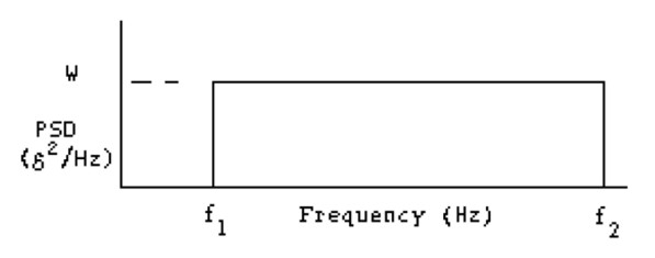
Figure 2: exempe of random excitation
The overall input Grms is the square root of the area under the curve, i.e.
Grms = √ w (f1-f2) (1)
This value could be used in Eq. 2 to predict the probability of occurrence of instantaneous values of acceleration for a random signal. For design purposes, Grms would generally be multiplied by three to provide three sigma values. To avoid the mechanical failure, the random vibration could be considered as:
a) an infinite number of harmonic vibrations with unpredictable amplitude and phase relationships in the frequency domain.
b) the sum of an infinite number of infinitesimal shocks occurring randomly in the time domain.
In the first case, response at a particular frequency may be the primary concern. For example, when a displacement sensitive device is excited at its natural frequency, relatively large displacements may result in malfunction. In such a case, the malfunction might be corrected by reducing the amplitude of excitation at the particular frequency of concern – the natural frequency of the device. This might be accomplished by inserting a vibration isolator between the source of excitation and the device. Alternatively, displacement might be reduced by adjusting the stiffness of the device, or by increasing damping at the natural frequency of the device. If the random vibration is considered as an infinite number of infinitesimal shocks, the overall Grms may result in a fatigue related structural failure of a component due to the intermittent shocks associated with the random excitation. In this case, the problem might be corrected by reducing the overall Grms or by increasing the strength of the component.
STATISTICAL ASPECTS
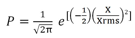
In random vibration, it may be necessary to predict the probability of a response for a exceeding particular value. For exemple, if a black box has a small clearance to an adjacent structure, it is ncessary to know the probability of the black box impacting the structure. Alternatively, since the probability of impact would never be absolutely zero, it would also be of interest to predict the average time between successive impacts, or the average number of times a particular amplitude may occur in a given duration. This would be of interest in calculating acceleration (or stress), and relating these values to the fatigue life of a component. The most commonly used probability distribution is the Normal (Gaussian) distribution. The probability density function for a normal distribution is give by:
 (2)
(2)
Equation 1 is plotted as Figure 3, which is the probability of occurrence of the ratio of the instantaneous value to the RMS value. In Equation 1, X and Xrms could have units of displacement, velocity or acceleration, or derivatives of these terms. The equation 1 could be used in equation 2 to predict the probability of occurrence of instantaneous values of acceleration for a random signal.
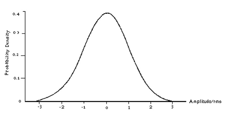
Figure 3: Normal (or Gaussian) distribution
For exemple, returning to the problem of the black box with a 0.25 inchs clearance to an adjacent structure, if Xrms were .0833 inches, the three sigma value would be .25 inches (3 x.0833), and the probability of impact would be .3% (the total area under the curve has value equal to 1.00 or 100%). The probability of impact could be reduced by reducing Xrms. For example, if Xrms were decreased to .0625, a four sigma deflection would be required to cause impact, and the probability of impact would be reduced to .001%.
A decibel is a logarithmic notation for expressing ratios between two quantities. For Power Spectral Density (g2/Hz), the following equation is used to relate two values of PSD:
ΔdB = 10 log [W1/W2]
An octave is a doubling or halving of frequency (e.g., 8 Hz and 16 Hz are separated by one octave as are 80 Hz and 160 Hz). Displacement are analyzed in the same manner as acceleration, except that rather than using units of g2/Hz, the units would be in2/Hz. For a band limited white spectrum, the RMS displacement can be shown to be given by:
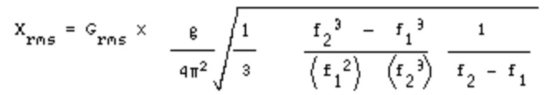
where,
Grms = input acceleration
g = acceleration constant= 386 in./sec.2
f1 = lower frequency, Hz
f2 = upper frequency, Hz
For most cases, f2 is significantly higher than fl and Equation 4 can be approximated by:
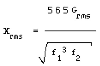
The last 2 equations could be used in conjunction with Equation 2 to determine the probability of occurrence of a particular input displacement.
ISOLATION OF RANDOM VIBRATION
If a mass supported on vibration isolators is subjected to a stationary, Gaussian random vibration input, the response will be a stationary, Gaussian random response. The use of vibration isolators could change the amplitudes of response, such as Power Spectral Density and Grms. The Power Spectral Densities of the isolated equipment (response) can be connected to the input by the following equation:
Wout=Win T2A
where, Wout = Power Spectral Density on isolated equipment
Win = Input Power Spectral Density
TA= Absolute Transmissibility of Isolation System
Insertion of vibration isolators modifies the frequency response to a random vibration input in a similar manner to a sinusoidal vibration input, because in sinusoidal vibration, there is a frequency region of amplification and a frequency region of attenuation. Even if the insertion of vibration isolators modifies the frequency response to a random vibration input in a similar manner to a sinusoidal vibration input, in random vibration, the amplitude of the response is modified by transmissibility squared, whereas, in sinusoidal vibration, the response is a linear function of transmissibility. This difference is due to the fact that in random vibration, we deal with power, whereas, in sinusoidal vibration, we deal with acceleration.
The RMS acceleration (Grms) transmitted to the isolated equipment is equivalent to the square root of the area under the curve of the response Power Spectral Density (g2/Hz):
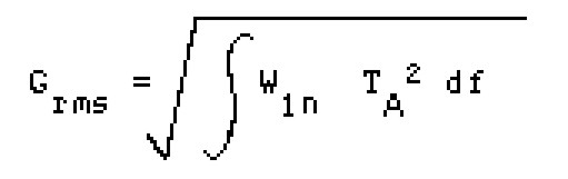
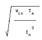
For a band limited white spectrum, this equation can be simplified to the following:
![]()
where, fn = Isolation System Natural Frequency, Hz
TA= Absolute Tranmissibility
Win = Input Power Spectral Density, g2/Hz
To calculate the relative displacement of a component to ensure tha sufficient clearance, based on two directly measureable parameters – Grms and fn, we can use this formula:
δrms = 9.75 Grms / fn2
If the random vibration excitation is a band limited white spectrum, the RMS displacement can be determined from:
The RMS displacement is typically multiplied by three to determine the minimum clearance required to prevent metal-to-metal contact. Could be necessary to estimate the average number of occurrences (N) of a particular event in a given time duration ( t). For a band limited white spectrum, the average number of occurrences in a given time duration can be estimated by:
N = 2 fn Δt e[(-1/2)(X/Xrms)2]
where, fn = Natural Frequency, Hz
Δt = Time Interval, Seconds
X/Xrms = Amplitude Ratio
For instance, if a black box has a 0.25 inch clearance (X), and if Xrms (also d rms) is .0833 inches, a three sigma deflection will cause metal-to-metal contact. If the isolation system natural frequency is 25 Hz, there would be an average of 33 impacts in a one minute period. If Xrms were reduced to .0625 inches, the average number of impacts in a one minute period would be reduced to one.
Fatigue Analysis of the vibrations.
For fatigue life calculation the root mean square (RMS) stress quantities are used in conjunction with the standard fatigue analysis procedure. Considering the Wohler curve of the stress-cycle, the approximate number of stress cycles N1 required to produce a fatigue failure in the beam for the 1σ, 2σ and 3σ stresses can be obtained from the following equation:
N1=N2(S2/S1)b
N2 = number of cycles for the stress reference point
S2 = stress reference point, to fail at N2
S1 = 1σ RMS stress
b = slope of fatigue line
Somethimes the b parameter has to consider the stress concentration K, for example if we are nearby a hole. Then it is necessary to calculate the number of fatigue cycles (n) accumulated for 1σ, 2σ and 3σ. To calcultate the remain life, can be used the Miner’s Rule that provides a reasonably good prediction.
NASTRAN Random Vibration Example
Following is an example of an MSC Nastran random vibration analysis run. The NASTRAN cards necessary to perform a random run are described here. The model is a Bracket monted on a crossbeam. This method is extremely similar to the frequency response runs.
Input Data Deck
$ RANDOM ANALYSIS
SOL 111
Modal Frequency Response Solution Number
$
TIME 10
CEND
$
TITLE = RANDOM VIBRATION EXAMPLE MODEL
SUBTITLE = Braket
LABEL = Y-DIRECTION RANDOM INPUT OF 0.01 G^2/hZ FROM 20-2000Hz
ECHO = NONE
$
SPC = 1
METHOD = 1
DLOAD = 10
SDAMPING = 20
RANDOM = 30
FREQ = 40
SPC refers only to the SPC1 card (not the SPCD card);
METHOD refers to EIGR card;
DLOAD refers to RLOADx card;
SDAMPING refers to TABDMP1 card;
RANDOM refers to RANDPS card;
FREQ refers to all FREQx cards used
$
ECHO = NONE
$
$SET 99 = 61629341
$SPCFORCES(PHASE) = 99
The preceding two cards are used for shaker point force recovery only (remove $ if needed).
SET 99 sets the shaker GRID 61629341 output;
SPCFORCES requests force recovery at SET 99 (see OUTPUT and SPCD cards below)
$
OUTPUT(XYPLOT)
XYPEAK,XYPUNCH,ACCE,PSDF/ 61629341(T2), 61630495(T2)
Cards used for plot output.
NOTE: THIS IS THE ONLY WAY TO GET RANDOM OUTPUT!
OUTPUT card is required to use XYPLOT commands;
XYPEAK recovers RMS and other peak responses in the .prt file (required for RMS output);
XYPUNCH creates a .pch file of response vs. frequency;
ACCE requests acceleration output (FORCE requests force output);
PSDF requests output as PSD;
GRID point 61629341 and 61630495 responses recovered; T1=X, T2=Y, T3=Z, as well as R1, R2, and R3
$
BEGIN BULK
$
PARAM,AUTOSPC,YES
PARAM,GRDPNT,0
PARAM,RESVEC,YES
PARAM,RESVEC,YES is REQUIRED for accurate results when NOT using the seismic mass. It computes residual vectors.
$
GRID 61629341 0 0. 0. 0. 0
Shaker grid point. Often this is an RBE element attached to many GRID points with the independent GRID being the shaker point.
$
SPC1 1 12345661629341
The Shaker point is SPC’d in all DOF
$
RLOAD2,10,11,,,12,,ACCE
RLOAD defines frequency response dynamic loading;
LOAD = SPCD * TABLED1 [= A * B(f)];
11 IS SPCD card;
12 IS TABLED1 card;
ACCE refers to type of dynamic excitation, enforced acceleration in this case. Other options are LOAD for applied load, DISP for enforced displacement, and VELO for enforced velocity.
$
SPCD,11,61629341,2,1.0
Y-axis input at GRID 61629341;
2 refers to input direction (1=X, 2=Y, 3=Z);
1.0 is any scale factor;
$
$SPCD,11,61629341,2,386.4
Use this card instead when recovering forces or displacements (assuming you’re using the inch/pound system), such as at the shaker point. If you’re using a metric based system, such as mm/gram, then 386.4 becomes 9807. (You can also change the 1.0 values in the TABLED1 card below to the acceleration value and get the same result. But do not change both.)
$
TABLED1 12 LOG LOG +
+ 20.0 1.0 2000.0 1.0 ENDT
TABLED1 is a tabular function defining the frequency-dependent portion of RLOAD2
The table is given as X1,Y1, X2,Y2, X3,Y3, etc.;
20.0 is the beginning frequency (X1); 1.0 is the magnitude (Y1);
2000.0 is the ending frequency (X2); 1.0 is the magnitude (Y2);
The Y values are used as scale factors; the actual Y values are entered as random input in TABRND1 below (not frequency input);
The LOG LOG entries refer to how the data is interpolated on each axis.
NOTE: All tables MUST end with an ENDT card.
Also, tables are not always compatible between UAI/NASTRAN and MSC/NASTRAN. The tables used in the older version of this example would not work under Nastran 2001.
$
TABDMP1 20 +
+ 20.0 0.1 2000.0 0.1 ENDT
Defines modal damping of Q=10;
The damping is 1/Q over the range of frequencies; in this case Q is constant. Q can vary over frequency if the proper data is available.
$
RANDPS,30,1,1,1.0,0.0,31
Defines random PSDF loading;
The important value here is the 31, which refers to the TABRND1 card
$
TABRND1 31 LINEAR LINEAR
+ 19.999 0.0015 200.0 0.09 2000.0 0.09 2000.1 0.01+
+ ENDT
Defines PSDF from 20 to 2000 Hz on a log-log scale;
First value must be slightly lower than actual frequency;
Format is Frequency, PSD,
Final value must be slightly higher than actual frequency
$
FREQ1,40,20.0,2.0,140
FREQ1,40,300.0,5.0,140
FREQ1,40,1000.0,20.0,50
FREQ3,40,20.0,2000.0
FREQx cards input frequencies where responses are recorded;
FREQ1 gives beginning frequency, freq. increment size and number of increments;
FREQ3 adds each natural frequency FROM 20 TO 2000 Hz
$
EIGRL 1 0. 2000. 0 MASS
EIGRL determines normal modes from 0 to 2000 Hz
$
INCLUDE ‘Bulk_DFEM.bdf’
Bulk Data can be elsewhere in a different file by include
$
ENDDATA
Example of a Random Vibration punch file output
Column 2 is Frequency, Column 3 is PSD response.
$ACCE 061629341 4 1.287988E+01 1.202460E+03 1
1 2.000000E+01 1.500034E-03 2
2 2.073522E+01 1.525330E-03 3
3 2.147043E+01 1.551055E-03 4
4 2.200000E+01 1.569851E-03 5
5 2.220565E+01 1.577211E-03 6
6 2.294086E+01 1.603809E-03 7
7 2.367608E+01 1.630856E-03 8
8 2.400000E+01 1.642917E-03 9
9 2.441130E+01 1.658360E-03 10
10 2.514651E+01 1.686326E-03 11
11 2.588173E+01 1.714764E-03 12
12 2.600000E+01 1.719383E-03 13
13 2.661695E+01 1.743681E-03 14
14 2.783382E+01 1.792619E-03 15
15 2.800000E+01 1.799408E-03 16
16 2.905069E+01 1.842931E-03 17
17 3.000000E+01 1.883158E-03 18
18 3.026756E+01 1.894654E-03 19
19 3.148444E+01 1.947831E-03 20
20 3.200000E+01 1.970807E-03 21
. . . .
. . . . . . . .
603 7.205206E+02 9.000000E-02 604
604 7.216171E+02 9.000001E-02 605
605 7.227136E+02 8.999999E-02 606
606 7.238102E+02 9.000002E-02 607
607 7.249067E+02 9.000002E-02 608
608 7.250000E+02 8.999999E-02 609
609 7.279968E+02 9.000002E-02 610
610 7.299999E+02 9.000000E-02 611
$ACCE 061630495 4 1.784084E+00 5.560125E+02 1568
1 2.000000E+01 1.796162E-03 1569
2 2.073522E+01 1.854036E-03 1570
3 2.147043E+01 1.915018E-03 1571
4 2.200000E+01 1.961002E-03 1572
5 2.220565E+01 1.979348E-03 1573
6 2.294086E+01 2.047296E-03 1574
7 2.367608E+01 2.119151E-03 1575
8 2.400000E+01 2.152129E-03 1576
9 2.441130E+01 2.195231E-03 1577
10 2.514651E+01 2.275887E-03 1578
11 2.588173E+01 2.361547E-03 1579
12 2.600000E+01 2.375826E-03 1580
13 2.661695E+01 2.452704E-03 1581
14 2.783382E+01 2.616812E-03 1582
15 2.800000E+01 2.640609E-03 1583
16 2.905069E+01 2.799714E-03 1584
17 3.000000E+01 2.957717E-03 1585
18 3.026756E+01 3.004980E-03 1586
19 3.148444E+01 3.237164E-03 1587
20 3.200000E+01 3.345061E-03 1588
.
.
603 7.205206E+02 1.264290E-04 2171
604 7.216171E+02 1.282528E-04 2172
605 7.227136E+02 1.301079E-04 2173
606 7.238102E+02 1.319973E-04 2174
607 7.249067E+02 1.339243E-04 2175
608 7.250000E+02 1.340897E-04 2176
609 7.279968E+02 1.395894E-04 2177
610 7.299999E+02 1.434853E-04 2178
Plot of the Example Random Vibration Data
Below is a plot of the data given in the punch file (random_test.pch). It shows the input and the response. The input is shown in figure 1. The response in general shows the peaks corresponding to the modes of the bracket.
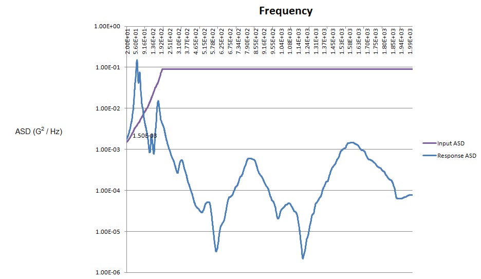
Figure 3: Normal (or Gaussian) distribution
One Response to Random Vibration Analysis – Nastran SOL 111