1 – Introduction
2 – Aerodinamic for compressible gas – Basic principles
3 – Performance of Jet Engine
4 – Turbogas cycle
5 – Turbofan
5.1 Turbofan with separated flows
5.2 Turbofan with associated flows
6 – Combustion chamber
7 – Inlet
8 – Nozzle
9 – Turbine Engine
In the study of systems propulsion, it is necessary identified performance indices capable to measuring in general features and performance engine itself. These quantities should indicate how an engine is able to carry out its task, and how is efficient. They must also allow comparison between different engines. The key variable in aerospace propulsion is the thrust, that is the force that the engine is capable of developing by supplying energy and accelerating the propulsive fluid ( air for turbofun or the product of the combustion of propellants fully stowed on board in case of the rocket).
The equations that are used to assess thrust and efficiency of an engine can be obtained simply from the equations of conservation of mass, quantities momentum and energy without to deepen into the details of the operation of systems characterizing each motor.
3.1 Thrust
The thrust can be obtained by increasing the quantities momentum of the incoming air processed by the engine. The air velocity is an important variable that can be neglected in the case of rockets. In the figure below is shown an jet engine in a wind gallery to simulate the flight condition (V0= velocity of air flow, V control volume, S control surface).
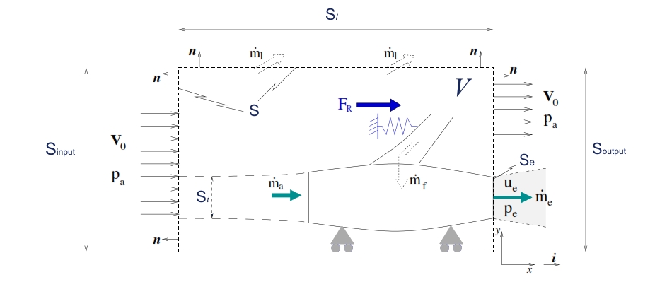
Fig. 10 : Control volume to extrapolate the thrust for an jet engine within an air flow with velocity V0
For the control volume considered are valid the principles of conservation of mass and the quantities momentum. For the conservation of mass in the motor entering a mass flow of air ṁa, and a fuel flow rate ṁf. which, after appropriate processing are ejected from the nozzle.
In stationary conditions the flow ejected from the nozzle is then:
![]()
In the control volume comes, by the surface Sinput , the air flow rate ṁin, which goes out by the lateral surfaces Sl , with flow rate ṁl (in this case is considered as positive) and by the surface Soutput, with flow rate ṁout. A part of the incoming flow from the left section passes through the engine, as well as that emerging from the right section includes that which has passed through the engine. As the incoming flow in the control volume must also consider the flow fuel ṁf.
The mass balance is written thus:
![]()
then separating the part of flow air that is not incoming in the engine, we have:
![]()
Consequently, the conservation of mass for the air flows around the engine requires:
![]()
The resultant of the forces acting on the control volume must be equal to the variation in the flow of momentum through it. This condition can be written:
![]()
The forces acting on the control volume are the reaction FR which must be applied to keep fix the engine, that is exactly equal to the thrust F, and the pressure forces acting on the control surfaces:

FR ≡ F ≡ Thrust
Air enters from the surface Sinput with velocity V0 perpendicular to the surface itself, and with
pressure equal to p0. The flux acting on Sl (lateral surface) has environmental pressure, velocity V0 parallel to the considered surface (unless to a small component perpendicular due to a small incoming and outcoming mass). By Soutput the flux is ejected. With regard to the Soutput, for the most of this surface (Soutput – Se) the flux features can be considered equal to the external one (V0 perpendicular to the surface, p=pa), whilst with regard theSe (the exit flow of the engine) we have pe and ue, with flow velocity perpendicular to the control surface as well. Since the pressure force related to Sl are applied perpendicular to the Thrust (n·i=0), the integral is equal to zero, and then the second term of (9) can be write:

The integral related to Sinput + Soutput is equl to zero. Therefore, grouping terms of (8) to integrate long Se and indicating with Ae the area of the surface Se, we have:
![]()
where the last eqution is obtained by noting that on this surface n ≡ i, and that the pressure p is uniform and equal to pe at the section of exit flow for the hypothesis of quasi-one-dimensional flow.
Regarding the variation of momentum, the second term of (8), it is observed that assuming a steady flow as hypothesis, the term in which this is the time variation of the quantities in time within the control volume is nil. It therefore remains to examine the flow of quantities momentum through the surface control that, by decomposing it into Sinput, Sl and Soutput, we have:
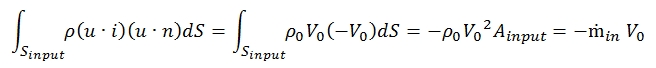
Note: n is directed in the opposite direction of i , whilst u=V0 i . The product od density, area and velocity is equal to the flow mass rate entering the control volume through the surface Sinput (with area Ainput).
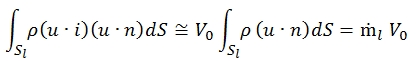
Regarding the second term of (11), although in the approximation in which u is directed as i, should not be present a mass flow and momentum through Sl , in realty by the equation of mass conservation is found that there is a flow of mass (positive if outgoing) denoted by ṁl.
The flow coming out from the control volume will bring away the corresponding momentum that can be approximated by:
The last term in the second member of (11) must distinguish the portion of Sout through which flows the air that has not passed through the engine from that Se where it passes the flow rate that instead has gone through the engine:

Substituting the results obtained in (10) we have:
![]()
From this equation we can obtain a simple equation for the thrust, by the equation saw before:
![]()
we have:
![]()
This is the Uninstalled Thrust, it is the thrust generated by the engine in case when the only force acting externally is the atmospheric pressure. Indeed during the flight is necessary to consider the interaction of the aircraft with the surrounding air, for this reason the hypothesis of constant pressure for surfaces Sinput, Sl, and Soutput – Se, is not anymore valid. Therefore the thrust obtained by (12) is lesser for a engine mounted on an aircraftby a drag factor due to the installation Dinst , that can be write as fraction φe and the unistalled thrust F:
![]()
Having separated the resistance of installation Dinst, which depends on the external encumbrance of the motor and its interaction with the body of the vehicle, one may therefore consider Uninstalled Thrust as a characteristic of the thurbofun. In fact the terms of the external forces which depend on the velocity flight in the aerodynamic forces are considered as dependent by the outside of the engine.
Wanting to study the characteristics of the engine from now on we riferir`a at the end thrust intending always pushing “non-installed”. In the our study we will consider only the Uninstalled Thrust.
Introducing the dilution ratio (ratio of the mass flow of fuel and the flow rate air that flows through the engine) f= ṁf / ṁa, we have for the thrust:
![]()
The first term is proportional to the flow discharged from the nozzle and the velocity of effluent ( jet thrust). The second term, negative, equal to the product of flow air introduced through the dynamic intake and the speed of flight, takes the name of resistance flight (ram drag). The third term name pressure thrust, is equal to the product of the effluent section and the difference between effluent pressure and the environmental pressure. Since the maximum allowable temperature in the turbine is limited, the f << 1 (generally f < 2%), therefore we can write with good approximation:
![]()
We can also introduce a speed of equivalent effluent:
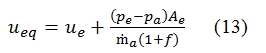
If the velocity effluent is subsonic or supersonic and such that pe=pa , then ueq=ue. Thus we can have:
![]()
The pressure term is important only if the nozzle works with choking condition (sonic flux in throat), whilst is nil if the effluent flux is subsonic. The presence of V0 implies that is important to specify the flight velocity for the thrust. Often the turbofun is studied with V0=0 and thus F=ṁaueq, this condition is named “tout-court”. The best condition to obtain the maximum thrust is that with pa=pe.
3.2 Power and Efficiency
To evaluate the performance of a propeller, in addition to knowing the thrust that it is able to generate,
must be able to assess the cost of this thrusting. The cost depends to the cost of source energy used and to the efficiency of the transformation of the power available in propulsive power.
Whether we consider the engine that uses the chemical energy as a source, the initial available power, is built up by two terms: the first is proportional to the product of the fuel flow rate and and the energy that It may be
supplied by burning the unit mass of fuel. The second is given by kinetic energy belongs the fuel for the fact of being on board the vehicle (which is in motion). Therefore the available power is equal to:
![]()
Where Qf is the power heat of the fuel (the energy needed to burn a unit mass of fuel). The term V02/2 can be neglectable with respect Qf.
This energy is provided to the propulsive fluid that is then accelerated. In this transformation occurs inevitable losses related to the performance of the thermodynamic cycle, as well as to the fact that in reality, not all the power supplied from the cycle is converted into propulsive power. As is shown in the figure below, the engine transform the available power in Pj (Power of the Jet) .
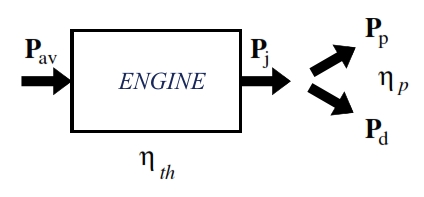
Fig 11 – power engine
The power that the engine gives the propulsive fluid corresponds to the variation of kinetic energy per unit time, and it is named jet power PJ. A percentage of this power is transformed in propulsive power Pp (the thrust has to balance the drag), that is equal to:
![]()
We must consider that the air flow is expelled from the engine with an kinetic energy which had not initially, indeed a part of this energy is lost. This is the residual or dissipated power Pd, it is the power not used to accelerate the flow (residual kinetic energy). The Pd can be calculated multiplying the residual kinetic energy (per unit mass) for the fuel flow rate:
![]()
In the equation of dissipated power Pd has been assumed that the jet flow expelled has its entire energy as the velocity. In realty when the nozzle in not “adapted” (i.e. when the flow jet is ejected to subsonic velocity, or when the nozzle does expansion of flow in supersonic regime exactly till to pressure equal to atmospheric pressure) we must consider the difference between the jet flow pressure and the atmospheric pressure, therefore the Pd is higher for a term proportional to pe-pa. To calculate correctly the Pd taking into account the pe-pa, we have to replace the ue with ueq (13). The power of the jet can be expressed as the sum of propulsive power and the dissipation power:
![]()
By the (16), (17), (12 b) we can write:

Once introduced then the equations for the powers involved in the various transformations, we can now introduce the efficiencies, which are defined as the ratios between powers and they are a measure of fraction of power that is found at downstream of a transformation than that which had upstream.
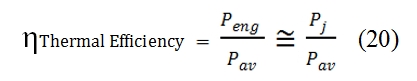
3.2.1 Thermal Efficiency
The thermal efficiency is the efficiency of the engine to convert the chemical energy in usable energy for the propulsion. It is not correlated with flight condition, is a measure of thermodynamic efficiency. The available power at downstream Peng, after the passage in the combustion chamber, decreases due to the losses for mechanical efficiency, efficiency of fan, frictions, etc. As first approximation we neglect these power losses, and we assume that all this power is provided to the jet flow as kinetic energy. Therefore, as approximation, we consider the efficiency as:
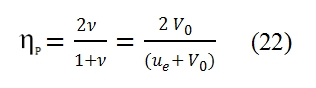
3.2.2 Propulsion Efficiency
The propulsion efficiency ηp is a measure of how much energy developed is used effectively to create thrust propulsion. This efficiency can be calculated as:
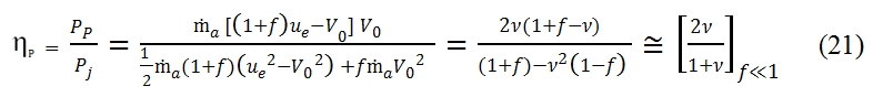
The propulsive efficiency equation can be simplified by introducing the ratio between the flight velocity and effluent velocity : ν=V0/ue. This ratio is always lesser then 1, otherwise we have not the thrust (see (14)) . In fig 12 is shown the trend of propulsion efficiency versus ν=V0/ue . This trend is equal for turbohelix and turbofan only when it is negligible the fuel flow rate with respect the air flow rate developed by the engine (this condition is verified with f<<1, fig 12). In the (21) the last term is obtained for the hypothesis of f<<1, and for 0≤ν≤1 the propulsive efficiency is an increasing function of ν, it is nil for V0=0, and it is equal to 1 with ν=1 (V0=ue). The condition V0=ue is verified when the residual kinetic energy is nil, but it is not possible because with ν=1 the thrust is nil as well. In fig 12 is shown the trend with f=0.05. It is very similar to that with f<<1, thus the hypothesis and formulas previously explained are still valid in general. It is important to evaluate the propulsive efficiency as function of flight velocity, and thrust. To obtain this link between these important parameter we have to consider the following equations:
Then from (14) we can write ue as function of F, ṁa, V0:
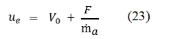
Therefore we have:
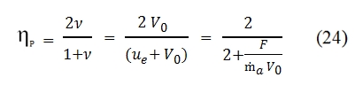
The ṁa is the flow rate that goes through the the engine. In fig 13 is shown the trend of propulsion efficiency versus F/ ṁa V0 , by this chart is clear that increasing the incoming air flow rate we can obtain an higher propulsion efficiency. Since the thrust is proportional to the incoming air flow rate and to its velocity variation due to the engine, to obtain higher propulsion efficiency is convenient to operate with bigger incoming air flow rate and with small velocity variations (ν=V0/ue is higher for ue lesser). As per the equation (21) we have the maximum efficiency with ν=1 and ηp=1 (with this assumption the residual kinetic energy is nil).
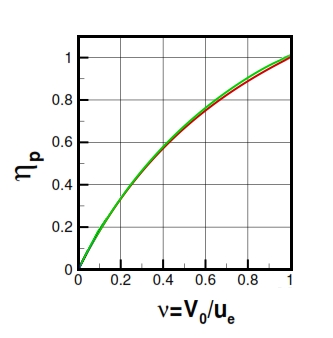
Fig 12. Propulsion efficiency versus ν=V0/ue, green line for f=0.05, and red line for f<<1.
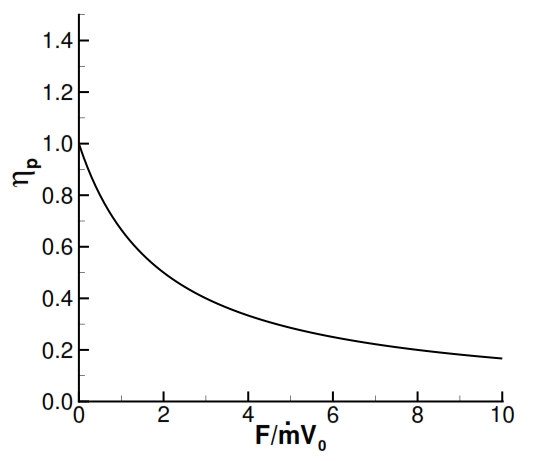
Fig 13. Propulsion efficiency versus the thrust
3.2.3 Global Efficiency
The global efficiency ηo gives an estimation of the percentage of the available power is converted in thrust power. Thus we can write the global efficiency by this equations:
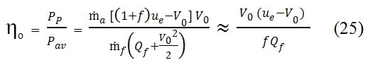
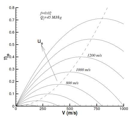
Fig 14. Global efficiency versus flight velocity and effluent velocity ue
With the assumption of f<<1 and with the hypothesis of V02/2<<Qf, we can simplify the equation (25). In this case we can observe an parabolic trend of the global efficiency proportionally to the V0. By deriving the (25) per f, with Qf and ue fixed, the global efficiency is biggest with V0= ue/2. Nevertheless in the realty f and ue are not constant with the variation of flight velocity, therefore this result is not true in general. Another aspect is that the ηo grows by decreaseing the f, that means a decreasing of fuel mass used for the combustion, but with this condition we have a decreasing of ue.
3.3 Specific Consumption
It is one of the most important parameter to measure the performances of the engines, and it gives a measure of how much fuel is needed to consume for the unit time to obtain the required performances. Usually as required performance is used as reference the thrust developed by the engine. This parameter depends very much from the flight condition. The specific consumption can be expressed with this formula (referred to the thrust):
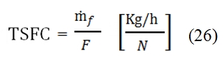
Thrust Specific Fuel Consumption
The TSFC for the Turbofan usually has a range value of 0.03 ÷ 0.05 (Kg / h) / N
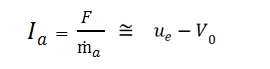
3.4 Specific Thrust
It is the thrust provided to the air for unit of flow rate. It is a sort of measure of the intensity of jet flow and provides an evidence of proportionally between the thrust and air flow rate, it can be write as:
(27)
The specific thrust for the Turbofans usually has a range value of 500 ÷1000 Ns/Kg. The specific thrust is inversely proportional to propulsive efficiency.
3.4 Autonomy
The autonomy of the Turbofan is equal to the maximum distance that the aircraft is able to cover (aircraft
range). This kind of parameter is related not only to the engine, but to the engine-aircraft coupling. For instance, if we suppose to consider an aircraft with constant flight altitude and constant velocity, the thrust has to be equal to the drag, thus:
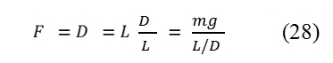
Since the overall efficiency is equal to:
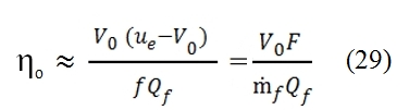
We can write:
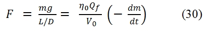
Where ṁf is equal to the variation of aircraft mass per unit time (dm/dt<0). By assuming that g, ηo, Qf, V0, and the aerodynamic efficiency E=L/D are constant, by the (30) we can write:

Thus the autonomy s can be expressed by this formula:
![]()
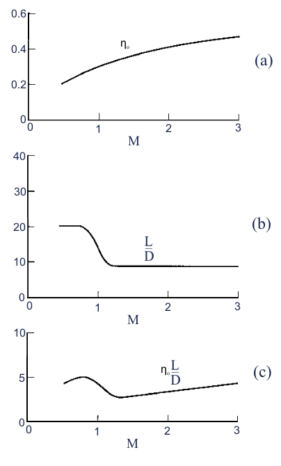
Therefore the fuel mass ṁf needed to cover the distance s, decreases only if we have a decreasing of the overall efficiency ηo or / and and the aerodynamic efficiency E. From the figure 15 we can observe that to obtain an high efficiency is necessary an high flight velocity. Due to the abrupt decreasing of the aerodynamic efficiency at the transition from subsonic field to supersonic field (Fig 15 b), we have maximum autonomy at velocity slighter lower of the sonic one (Fig 15 c).
For this reason the most aircrafts of the airliner companies fly with Mach ~ 0.85. To obtain an equivalent high efficiency, the Mach number has to be bigger to 3, with problems related to the material due to heating (the aluminum softens at few hundreds of celsius degrees, should to be used the Titanium or the Steel, but are heavier than the aluminum) , aerodynamic configuration (the stability is more difficult at high Mach number, and we have lesser manoeuvrability), sonic shock, costs.
[smartslider3 slider=”2″]