1 – Introduction
2 – Aerodinamic for compressible gas – Basic principles
4 – Turbogas cycle
5 – Turbofan
5.1 Turbofan with separated flows
5.2 Turbofan with associated flows
6 – Combustion chamber
7 – Inlet
8 – Nozzle
9 – Turbine Engine
The Turbofan creates power propulsion by the turbogas cycle. From the theory, a thermodynamic cycle is a method to provide or obtain energy by means exchange with a fluid, which is used as energetic vector. By the study of the thermodynamic cycle is possible to evaluate the performance parameters (Thrust, Power, Specific Consumption) on depending of the project requirements (for instance the maximum operative temperature of turbine), of flight operative conditions (temperature, environmental pressure, Mach number), and project aims (compression ratio of compressor, bypass rate, compression ratio of fan, etc..). Hereafter the cycle analysis is argued by considering the several components as “black box” without to analyse in deep their functionalities, considering their global effects they produce. In the thermodynamic cycle the fluid mass is subjected to cyclic transformations, at each cycle end, the fluid will be at same condition of beginning, the same before the starting of cycle. To study these transformations, is enough to know just two state variables if the fluid is monophase. For this scope is used the Clapeyron plane p-v, where for a reversible transformation, the area inglobed into the curve is equal to the work exchange (used mainly for alternate engines). Another important method are the Mollier plane h – s and the entropic plane T – s.
The turbogas cycle is also called the Joule-Brayton, and is studied on the plane h – s or, if can assume constant the specific heat (as assumed in these hereafter), on the plane T – s, see Fig. 16., since we have a continue flux. In Fig. 16 is represented also the diagram of the cycle in the plane Clapeyron. In the plane T – s the slope of a curve, that represent a transformation, it may be inferred from the relationship of Gibbs: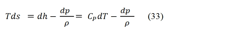
For an isobaric transformation we have:
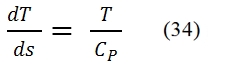
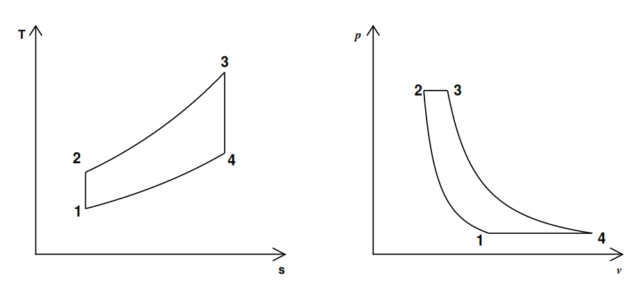
Fig 16. ideal turbogas cycle
The cycle gas turbine describes the evolution of the state of a mass fluid, divided into four phases, the which allows to transform part of the heat that is administered to the fluid into work. It consists of the following transformations:
1-2 Isentropic compression. The fluid is compressed in the first phase. This transformation that ideally takes place without heat exchange (adiabatic trasformation) and in a reversible manner (adiabatic reversible, thus isentropic). The compression also causes a temperature increase and a reduction of specific volume. The fluid is compressed with the scope to produce work, by expansion after it has been energized for the heat exchange.
2-3 Adduction heat at constant pressure. In this transformation the involute fluid mass receives heat from the outside. This process can occur in several ways. In the case of the Joule-Brayton cycle, ideally it occurs at constant pressure. Obviously the supply of heat leads to an increase of the temperature and, since it takes place at constant pressure, even an increase of the specific volume v. At this stage no work is exchanged with the outside.
3-4 Isentropic expansion. Likewise the compression, this transformation is actually carried out without heat exchange with the outside (adiabatic) and in a reversible manner (isentropic). By means the expansion the fluid, carries out work and its temperature decreases, whilst its specific volume increases.
4-1 Heat dissipation with constant pressure. The fluid, having recovered the initial pressure at the end of the previous transformation, but yet is still at a higher temperature than the initial one (since not all the heat supplied can be transformed in work, for the second principle of thermodynamics), must be cooled to return to initial conditions. Also this process is performed without exchanging work with the outside.
The ideal cycle described is a “closed” cycle (the operating fluid at the end of the cycle starts with a new one); it is also assumed that the heat is exchanged with the fluid through ideal heat exchangers.
However, in practice this cycle represents quite well the evolution of a cycle “open” in which the mass fluid is first compressed (1 -2), and then increases its temperature through the transformation of chemical energy into thermal energy (combustion, 2 – 3), and then expands providing work (3 – 4). The transformation that brings the fluid in the initial state takes place outside the engine, as the fluid ejected in 4 conditions gradually returns in thermal equilibrium with the environment. A scheme is shown in Fig. 17.

Fig 17. Scheme of a gas turbine
where the work is to supplied to the fluid by the compressor C, and heat through combustion that takes place in the combustor (Burner) due to the introduction of fuel. The fluid then expands in the turbine T, providing the energy necessary to set in motion the compressor, the excess energy is exploited by the user (P). In this open-loop, the properties of the involute mass fluid is modified due to effect of combustion (in particular, the oxygen content decreases) for which must renew it at each cycle. Strictly then the process is not more to consider as cyclical but as continuous process, in which each fluid particle follows the evolution 1-4.![]() The L and Q have positive sign if they are provided to the fluid. Hereafter with L´s and Q´ we denote work and heat, in the equation (35) they are expressed per unit time (power), instead by means L and Q respectively denote work per unit mass and heat per unit mass. Thus the 4 phases can be represented with these equations:
The L and Q have positive sign if they are provided to the fluid. Hereafter with L´s and Q´ we denote work and heat, in the equation (35) they are expressed per unit time (power), instead by means L and Q respectively denote work per unit mass and heat per unit mass. Thus the 4 phases can be represented with these equations:
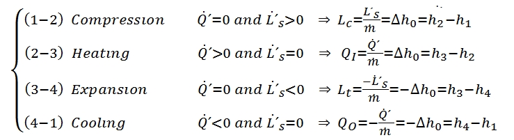
(36)
For the Compressor the work Lc is considered positive if it is furnished to the fluid, for the Turbine the work L is positive whether it is produced by the fluid. In (36) with QI and Qo are rispectively the heat incoming in the combustor, and the outcoming heat due to the cooling phase with production of exhaust gases. Both are positive for the combustion and for the discharger.
4.1 Ideal Cycle
By means the study of the ideal cycle we can evaluate the maximum limit of the engine performances for a real cycle. For this study we make the following assumptions:
- Ideal Gas: we assume an ideal behavior of the gas; the equation state P=ρRT is valid and Cp and Cv and thus ϒ are constant.
- Frictions and heat dissipation are assumed negligible: The friction implies as consequence a reduction of the total pressure, which is neglected.
- Pressure dissipation is negligible: the adding and subtraction of heat to the fluid imply the total pressure changes. By this hypothesis these variations are negligible.
- Adiabatic and reversible expansion / compression (isentropic trasformations)
- Mass variation is assumed negligible: the mass is constant, without any adding of the fuel, neither for dissipations.
- Constant chemical composition: in the realty this changes due to the addition of the fuel, and for the successive reaction. Nevertheless this mass is a small fraction of the air flow rate, therefore the chemical variation with the consequent molecular weight variation are negligible.
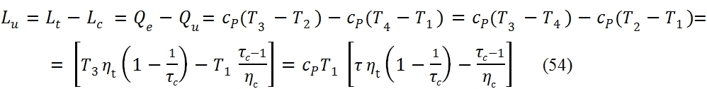
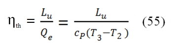
The performances with these hypothesis are obviously better than the reality ones. The thermodynamic efficiency ηth is the ratio between the useful work Lu of the fluid per unit mass, and Qe heat provided to the fluid per unit mass. The useful work is the difference (per unit mass) between that produced in the turbine and that absorbed by the compressor:
Lu = Lt – Lc
Since for the hypothesis assumed the fluid has the same initial properties at the end of every cycle, we have:
![]() Thus the ηth can be written:
Thus the ηth can be written: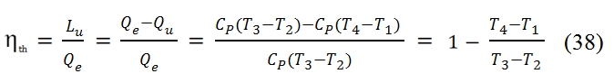
The formula (38) can be simplified because the cycle has two equal couple of transformations (two isentropic, and two isobaric). By introducing compression ratio βc = p2/p1, and reminding the relationship between the temperature and pressure for an isentropic transformation, we can write:

As consequence we have:
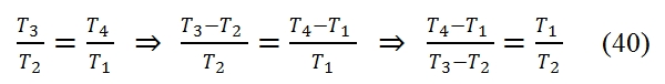
Thus by using the (40) and (39) in the (38), we have:
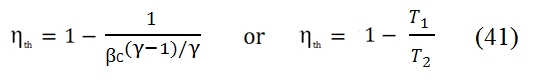 Therefore the efficiency does´not depend to temperature, but only of pressure ratio βc. It should however be noted that, fixed the temperatures T1 and T3 of the cycle, the compression ratio can not exceed the limit value:
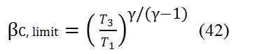
At limit the temperature at the end of the compression T2 is equal to the maximum acceptable temperature in the turbine T3. In figure 18 is shown the trend of the efficiency versus the compression ratio; we can note that it increases with βc.

Fig 18. Thermodynamic Efficiency versus Compression ratio, ideal cycle
Could be interesting to compare the cycle with the Carnot cycle, which is the maximum allowable (represented with dot line in Fig.19). The efficiency of Carnot is equal to: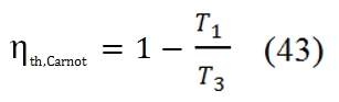

Fig 19. Ideal turbogas cycle versus Carnot (dot line) cycle with the same minimum and maximum temperatures.
To have the same efficiency, the maximum temperature T3 and the minimum temperature T1 have to be the same for both cycles, and to obtain identical curve, the transformation 2 – 3 and 4 – 1 have to occur at constant temperature. Another important aspect is the behaviour of useful work Lu (per unit mass). By T-s chart (fig 16), we can observe that Lu is proportional to the difference between the segment 3-4 and 2-1; indeed the first segment is proportional to Lt, because Lt is equal to Δh=cp ΔT in an adiabatic transformation, and the second one is proportional to Lc since this transformation is adiabatic as well. Therefore to have useful work Lu, must be Lt > Lc, i.e. with the same pressure ratio, the Δh has to be bigger in the turbine than compressor. The useful work Lu can be calculated by means the thermodynamic efficiency as well:
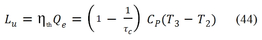
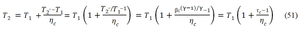
Where Qe is the heat furnished to the unit mass of fluid, and τc =T2 / T1. By considering the relation among T2, T1 and βc (or τc) (because the transformation 1-2 is isentropic):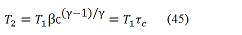
The useful work can be expressed as: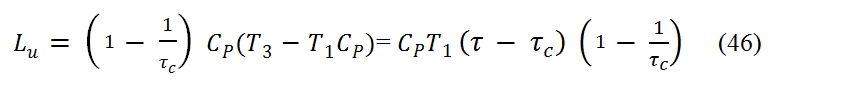
Where τ is the ratio between the maximum temperature and minimum:
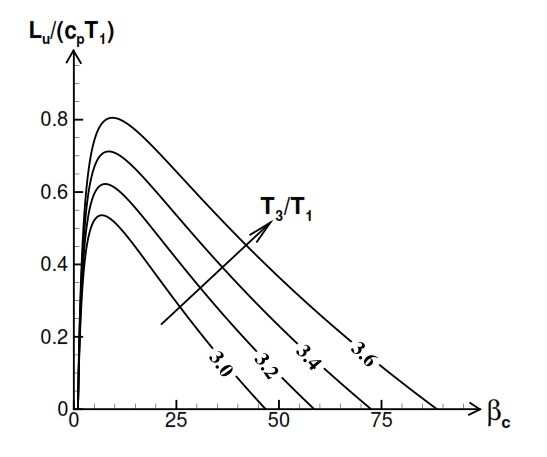
Fig 20. Trend of Lu versus compression ratio (βc) and versus the ratio between maximum temperature T3, and minimum temperature T1.
Therefore the Lu depends of the compression ratio βc and minimun temperature and maximum temperature (Fig. 20).
The Lu is equal to zere when:
- ηth =0, i.e. τc =1 (or βc=1); in this case we have no compression, that means the fluid doesn’t expand and doesn’t carry out work. Since Lu is equal to the area included to the cycle curve in the plane T – s, by the fig 21 we can deduce that Lu =0 when βc =1, since in this case T2=T1 and T3=T4.
- Qe =0, i.e. T3 = T2 then τc = τ; it is not provided heat to the fluid, as consequence in the expansion phase it has energy sufficient only to compensate for the compression work. This result It may be inferred by observing how it reduces the area of the cycles shown in Fig. 12, the evolution from left to right that corresponds to the growing of β
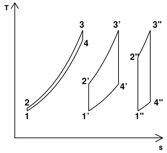
Fig 21. Turbogas cycles between two same temperatures for different values of βc (increasing values from left to right)
From Fig. 20 the Lu has maximum value for:
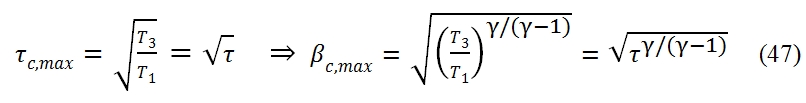
These equation can be obtained by calculating the value of τc (or βc) to obtain dLu/d τc=0. This result is due to the fact that, for assigned values of the maximum and minimum temperatures of the cycle, by variation of βc, the thermodynamic efficiency increases with the βc, while the heat that It may be supplied to the cycle decreases with the increase of βc, (because T2 is closer to the T3).
From the equation (47) is also observed that the value of the compression ratio, in correspondence maximum useful work, increases with the ratio τ = T3/T1.
Moreover the maximum value of useful work Lu occurs at T2=T4. Indeed in the ideal cycle we have: As consequence T4/T2 is equal to:
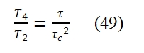
To obtain the maximum useful work Lu, must be τc= τc,max , then putting first equation of the (47) in the (49), we have: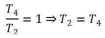
As well as βc, the useful work also depends on the value of T1 and T3 . The useful work Lu grows with the increase of the maximum temperature of the cycle T3 (or equal to the ratio of temperature τ, with fixed temperature T1); furthermore, increasing the T3 also extends the range of values of βc, that implies positive Lu (Fig. 20).
4.2 Real Cycle
For the study of the real cycle some hypothesis used for the ideal one are removed:
- Compression: it is assumed adiabatic, but not isentropic
- Combustion:
- The transformation is not isobaric
- The mass flow rate increases during the cycle (due to the fuel intake)
- The flux properties change during the cycle (due to the fuel intake and combustion)
- Heat loss (from the hot fluid to the engine)
- Introducing of combustion efficiency (to account for losses mentioned above, and incomplete combustion)
- Expansion: it is assumed adiabatic, but not isentropic
The deviation from the ideal cycle is represented in the plane T – s shown in Fig. 22, where the points marked with apex are relate to the ideal cycle, which it is characterized by the same compression ratio and from the same maximum temperature of the real one.

Fig 22. Real cycle of gas turbine
To highlight some essential aspects that distinguish the real from the ideal cycle, we consider an simplified study of the real cycle, where we do not remove all the hypothesis listed above and we make further following hypotheses:
- 1≡1´, whilst in the realty 1 ≠1´due to loss in the entrance of compressor ;
- The involute fluid is made up of air;
- The involute fluid is calorically perfect: cp(T)=const;
- The fuel flow rate injected is negligible compared to the air flow rate: ṁf <<ṁa
- The heat losses in the combustion chamber and due to incomplete combustion are negligible
Substantially, in this simplified study of real cycle we are focused on the reversibility of the fluid transformations in the compressor and in the turbine, neglecting the others real effects of lesser importance.
As consequence for these hypothesis we have p2=p2´ and 3≡3´.

Fig 23. Simplified real cycle of gas turbine
To compare the real cycle with the ideal one we consider some efficiency index by means we can measure how far the real cycle is close to the ideal one. For the compressor we consider the adiabatic efficiency defined as ratio of ideal work L´c needed to obtain the required compression ratio βc , and the work Lc really needed to obtain the same result. Since the transformation that occurs in the compressor is adiabatic, for the energy equation, the work depends by the variation of total enthalpy, hence depends of total temperature:

The point 2 and 2’ are on the same isobar p2= p2’= βc p1, but the real work exchanged Lc> Lc’, thus the temperature and entropy in 2 are bigger than in the point 2’.
Assuming the compressor adiabatic efficiency as known, the temperature at the exit is equal to this fundamental relationship:
Whilst for the pressure is valid this equation:
p2=βc p1
Similarly, the adiabatic efficiency of the turbine is defined as the ratio between the work extract in the reality Lt with an expansion rate βt=p3/p4 assigned, and the ideal one Lt´, with the same expansion rate. Thus the points 4 and 4’ are on the same isobaric curve p3=p4’= p3/ βt, but the work truly extracted is Lt < Lt´, hence the temperature value and the entropy values in the point 4 are higher than in 4’. Since the transformation is adiabatic (Lt = h03 – h04 ≃ h3 – h4) we have:

By the pressure ratio βt provided, the turbine temperature at the outlet can be calculated through the fundamental relationship:
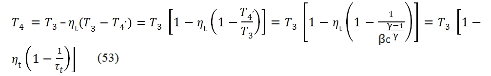
Where τt =βt(ϒ-1)/ϒ. The pressure at the outlet is obviusly equal to p4=p3/ βt. The area inside the curve T – s for the real case is not anymore the heat exchanged, thus the work is not proportional to cycle area, and whether we have a decreasing of the efficiencies of the compressor and turbine the useful work decreases, till the point that ever if βc > 1 and T3 > T2, the cycle could not provide useful work. The area inside the curve T – s is not anymore the heat exchanged because Lu is equal to the difference between the input heat and the output heat, which in the real case is bigger for the dissipation.
The useful work Lu for the real cycle (with τc = βc(ϒ-1)/ϒ the tempreature ratio for the isentropic transformation) can be calculated by the (51) and (53):
This quatity is reported for the real cycle (ηc=0.8, ηt=0.9) in fig. 24.

Fig 24. Lu versus βc for a gasturbine
And by using the (54), (46)´, (51) and considering the efficiencies, we have:
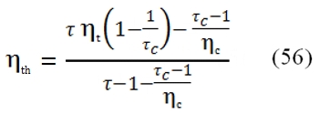
That is equivalent to write (ηth,id=1 – 1/τc for the ideal cycle):
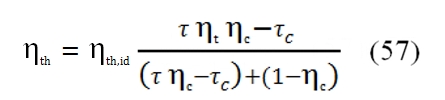
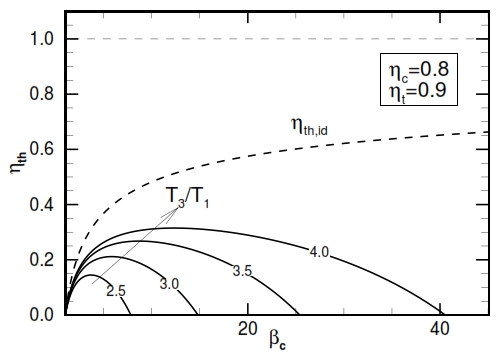
Fig 25. Thermodynamic efficiency for a real cycle
The trend of ηth is described by the figure 25. As can be observed by this graph, it have a maximum value, instead the ideal one grows only, and this maximum value increases with higher values of βc and τ. From this outcome is evident the necessity to have an high operative temperature T3 (the input temperature T1 can be supposed constant, it depends to by atmospheric condition). The turbogas cycle can be improved to obtain higher useful work or higher efficiency. On the other hand, these improvements can determine a relevant weight augmentation, not acceptable in the aeronautical field, where the lightness is very important.