[kofi]
[paypal-donation]
General Overview
There are many reasons to compute the natural frequencies and mode shapes of a structure. One reason is to assess the dynamic interaction between a component and its supporting structure. For example for those parts nearby the engines, is better to avoid that the natural frequencies of own part, fall in the vibration range of the engines, to avoid resonance problem. The solution of the equation of motion for natural frequencies and normal modes requires a special reduced form of the equation of motion. If there is no damping and no applied loading, the equation of motion in matrix form reduces to:
[M]{ü}+[K][u] = 0
Where
[M] = mass matrix
[K] = stiffness matrix
To solve this equation is assumed a harmonic solution:
{u}={φ} sin ωt
Where:
{φ} is the eigenvector or mode shape
ω is the circular natural frequency
The harmonic form of the solution means that all the degrees-of-freedom of the vibrating structure move in a synchronous manner. The structural configuration does not change its basic shape during motion; only its amplitude changes. By using the armonic solution in the differential equation, after simplifying it becomes:
([K]-ω2[M]) {φ}= 0
This equation is called the eigenequation, which is a set of homogeneous algebraic equations for the components of the eigenvector and forms the basis for the eigenvalue problem.
[A – λI] x =0
where:
A = square matrix
λ = eigenvalues
I = identity matrix
x = eigenvector
There are two possible solution forms for this equation
1) If det([K]-ω2[M])≠0, the only possible solution is
{φ}= 0
This rappresents the case of no motion
2) If det ([K]-ω2[M])=0, then a solution with φ≠0 is obtained,
det ([K]- λ 2[M]) = 0
where λ = ω2
The determinant is zero only at a set of discrete eigenvalues λi or ωi.
([K]-ω2[M]) {φ}=0
There is an eigenvector which satisfies the equation above and corresponds to each eigenvalue, thus this equation can be rewritten as:
([K]-ωi2[M]) {φi}=0 i = 1,2,3 …
Each eigenvalue and eigenvector define a free vibration mode of the structure. The i-th eigenvalue is related to the i-th natural frequency as follows:
fi= ωi/2π
where:
fi=i-th natural frequency
ωi = √ λi
The number of eigenvalues and eigenvectors is equal to the number of degrees-of freedom that have mass or the number of dynamic degrees-of-freedom. There are a number of characteristics of natural frequencies and mode shapes that make them useful in various dynamic analyses. First, when a linear elastic structure is vibrating in free or forced vibration, its deflected shape at any given time is a linear combination of all of its normal modes:
{u}= Σi(φi)ξi
where:
{u} = vector of physical displacements
(φi) = i-th mode shape
ξi = i-th modal displacement
Second, if and are symmetric and real (as is the case for all the common structural finite elements), the following mathematical properties hold:
(φi)T [M] (φj) = 0 if i≠j
(φi)T [M] (φi) = mj= j-th generalized mass – (orthogonality property)
and
(φj)T [K] (φj) = 0 if i≠j
(φj)T [K] (φj) = kj= j-th generalized stiffness = ω2mj (orthogonality property)
ωj2= [(φj)T [K] (φj)] / [(φj)T [M] (φj)
The orthogonality property of normal modes ensures that each normal mode is distinct from all others. Physically, orthogonality of modes means that each mode shape is unique and one mode shape cannot be obtained through a linear combination of any other mode shapes. A natural mode of the structure can be represented by using its generalized mass and generalized stiffness. For each possible component of rigid-body motion or mechanism, there exists one natural frequency that is equal to zero. The zero-frequency modes are called rigid-body modes. Rigid-body motion of all or part of a structure represents the motion of the structure in a stress-free condition. Stress-free, rigid-body Eq. 3-17 modes are useful in conducting dynamic analyses of unconstrained structures, such as aircraft and satellites. Also, rigid-body modes can be indicative of modeling errors or an inadequate constraint set. An important characteristic of normal modes is that the scaling or magnitude of the eigenvectors is arbitrary.
Mode shapes are fundamental characteristic shapes of the structure and are therefore relative quantities. In the solution of the equation of motion, the form of the solution is represented as a shape with a time-varying amplitude. Therefore, the basic mode shape of the structure does not change while it is vibrating; only its amplitude changes.
Although the scaling of normal modes is arbitrary, for practical considerations mode shapes should be scaled (i.e., normalized) by a chosen convention. In MSC.Nastran there are three normalization choices, MASS, MAX, and POINT normalization. MASS normalization is the default method of eigenvector normalization. This method scales each eigenvector to result in a unit value of generalized mass:
(φi)T [M] (φj) = 1.0
This method is appropriate to get a simplier computational and to reduce the data storage amount. In MAX normalization, each eigenvector is normalized with respect to the largest a-set component. This normalization approach can be very useful in the determination of the relative participation of an individual mode. A small generalized mass obtained using MAX normalization may indicate such things as local modes or isolated mechanisms.
POINT normalization of eigenvectors allows you to chose a specific displacement component at which the modal displacement is set to 1 or -1. This method is not recommended because for complex structures the chosen component in the non-normalized eigenvector may have a very small value of displacement (especially in higher modes). This small value can cause larger numbers to be normalized by a small number, resulting in possible numerical roundoff errors in mode shapes.
Modal quantities can be used to identify problem areas by indicating the more highly stressed elements. Elements that are consistently highly stressed across many or all modes will probably be highly stressed when dynamic loads are applied.
Methods of Computation
Seven methods of real eigenvalue extraction are provided in MSC.Nastran:
1) Lanczos Method
2) Givens method
3) Householder method
4) Modified Givens method
5) Modified Householder method
6) Inverse power method
7) Sturm modified inverse power method
The reason for seven different numerical techniques is because no one method is the best for all problems. The methods of eigenvalue extraction belong to one or both of the following two groups:
• Transformation methods
– Givens method
– Householder method
– Modified Givens method
– Modified Householder method
• Tracking methods
– Inverse power method
– Sturm modified inverse power method
In the transformation method, the eigenvalue equation is first transformed into a special form from which eigenvalues may easily be extracted. In the tracking method, the eigenvalues are extracted one at a time using an iterative procedure. The recommended real eigenvalue extraction method in MSC.Nastran is the Lanczos method. The Lanczos method combines the best characteristics of both the tracking and transformation methods. For most models the Lanczos method is the best method to use, It is the preferred method for most medium- to large-sized. The Givens and Householder methods are the most efficient methods for small problems and problems with dense matrices when a large portion of the eigenvectors are needed. The Householder method costs about half as much as the Givens method for vector processing computers. In addition, the Householder method can take advantage of parallel processing computers.
The modified Givens and modified Householder methods are similar to their standard methods with the exception that the mass matrix can be singular. Although the mass matrix is not required to be nonsingular in the modified methods, a singular mass matrix can produce one or more infinite eigenvalues. Due to roundoff error, these infinite eigenvalues appear in the output as very large positive or negative eigenvalues. The modified methods require more computer time than the standard methods.
There is also the Automatic Givens and Automatic Householder Methods, that they use the modified methods when necessary for numerical stability but use the standard methods when the numerical stability is accurate. The inverse power method is a tracking method since the lowest eigenvalue and eigenvector in the desired range are found first, its use is adapt to determine a few modes. Then their effects are “swept” out of the dynamic matrix, the next higher mode is found, and its effects are “swept” out, and so on. However, the inverse power method can miss modes, making it unreliable.
The Sturm modified inverse power method is a more reliable tracking method. This method is similar to the inverse power method except that it uses Sturm sequence logic to ensure that all modes are found. The Sturm modified inverse power method is useful for models in which only the lowest few modes are needed. This method is also useful as a backup method to verify the accuracy of other methods.
Entry for the Real Eigenvalue Analysis
Commonly the EIGRL entry is the most used method for the normal mode analysis:
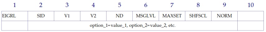
SID : Set identification number.
V1, V2 : lower and upper friquencies of the range of interest.
ND : number of the egenvalues and enginevectors desired
NOR: Method for normalizing eigenvectors, “MASS” (Default) or “MAX”.
MSGLVL (0 = Integer = 4; Default = 0): in some cases, higher diagnostic levels may
help to resolve difficulties with special modeling problems.
MAXSET (1 = Integer = 15; Default = 7): it is useful to set the memory size for the computation, a smaller block size may be more efficient when only a few roots are requested.
SHFSCL: When large mass techniques are used in enforced motion analysis (This analysis is used to ensure the quality of the model by applying a big mass and an enforced motion, generally as quality requirements are “rigid” displacements for the frequencies related to the enforced rigid motion, and “flexible” displacement for the rest) a large gap between the rigid body and flexible frequencies, which can degrade performance of the Lanczos method or cause System Fatal Message 5299. To avoid these problems, the SHFSCL can be used, its value should be set close to the expected first nonzero natural frequency.
The defaults on the EIGRL entry are designed to provide the minimum number of roots in cases where the input is ambiguous.
For the for the Other Methods:
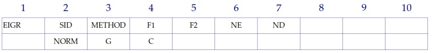
The METHOD field selects the eigenvalue method from the following list:
– AGIV Automatic Givens method
– AHOU Automatic Householder method
– GIV Givens method
– HOU Householder method
– INV Inverse power
– MGIV Modified Givens method
– MHOU Modified Householder method
– SINV Sturm modified inverse power method
The NE field is used by the INV method only. It defines the estimated number of roots in the range. A good estimate results in a more efficient solution. A high estimate helps to ensure thaall modes are computed within the range.
BDF Exemple:
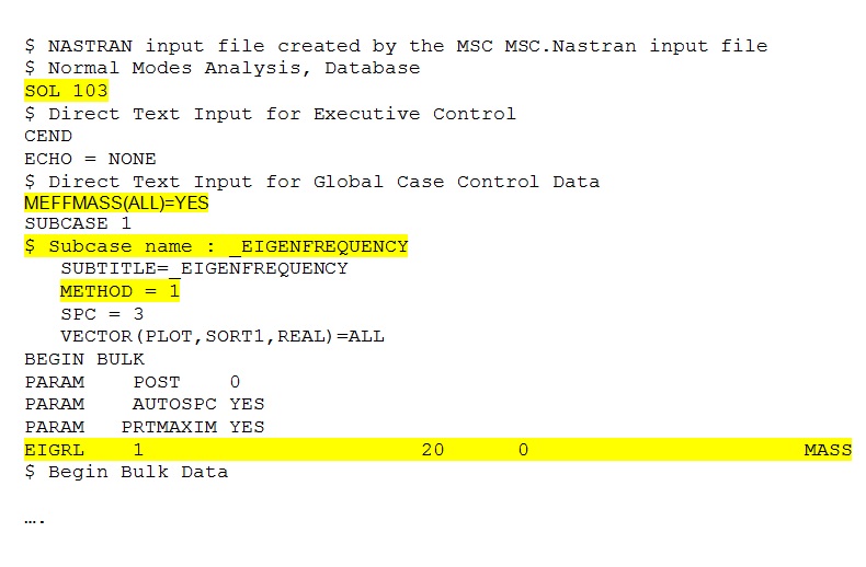
Obviously if you have a loaded model, the normal mode analysis has to be performed excluding the load applied, leaving only the constraints. The MEFFMASS sometimes can be useful to understand for each mode which fraction of the global mass is mostly involved. The results can be observed by the F06 file generated by Nastran (see below), in the “cycles” column there are the frequencies in Hz of the natural modes.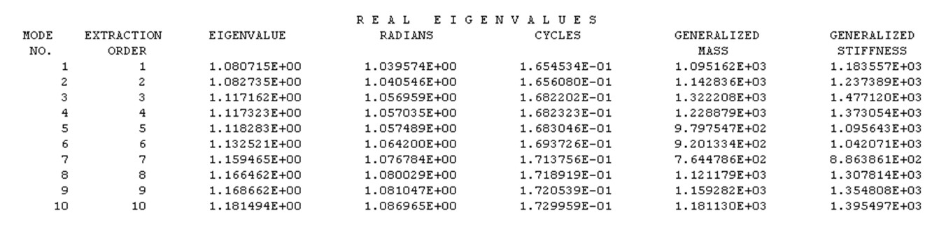
[kofi]
[paypal-donation]
One Response to Vibration Analysis – Nastran SOL 103