Buckling analysis assesses the stability characteristics of a structure. An accurate solution to a buckling problem requires more efforts than just following a numerical procedure, there are a number of factors to consider before a buckling solution can be accepted with confidence. A starting step should be a linear buckling analysis (see LINK). Nonlinear buckling analysis capability has been available in SOL 106 by restart. While serving the purpose of a nonlinear buckling analysis following a static nonlinear analysis, this buckling analysis procedure is cumbersome to the user because it requires a restart. To provide a more convenient and versatile capability for nonlinear buckling analysis, an option for a buckling analysis in a cold-start run with PARAM, BUCKLE, 2 was introduced in MSC.Nastran Version 70.7. This option allows a buckling analysis in any Subcase that has the METHOD command specified for an eigenvalue analysis. There are two more ways in nonlinear analysis to estimate the critical buckling load. One method is the arc-length method that can provide solutions past the critical buckling load into the post-buckling state.
Using the arc-length method, the nodal displacement of a point with the most noticeable motion should be traced to illustrate the peak point. The applied load at this peak resembles the critical buckling load. Another method is to use Newton’s method until the solution cannot be obtained due to divergence, in which case the adaptive bisection method is activated in the vicinity of the critical buckling load and stops at the limit load, close to the critical buckling point.
Plate Buckling Theory
An analytical calculation of the critical buckling load by use of the theory elasticity can be done in two ways, either by use of an energy method or by solving the differential plate equation. The plate differential equation or equilibrium equation looks as follows (Brush & Almroth, 1975):
![]()
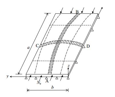
If a perfectly flat, rectangular plate that is simply supported along all four edges and subjected to a uniaxial compressive force in the x-direction, without any initial imperfections is assumed, the equilibrium equation takes the following form:

where w(x, y) is the out-of-plane deflection and D is the flexural rigidity. The out-of-plane deflection, w(x, y), can be described by a Fourier function series: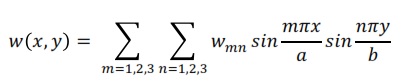
where m and n indicate the number of half sine waves in the two directions over the plate. This assumed sine function describing the out-of-plane deflection automatically satisfies the boundary conditions for a simply supported plate, as there are no deflections and bending moment (curvatures) at x = 0, x = a and y = 0, y = b respectively. By using this Fourier function series the following expression is obtained:
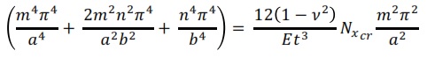
Rearranging this equation: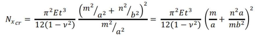
The lowest value of the buckling load is obtained for n = 1: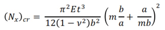
The critical buckling stress is obtained by dividing this equation with the thickness of the plate: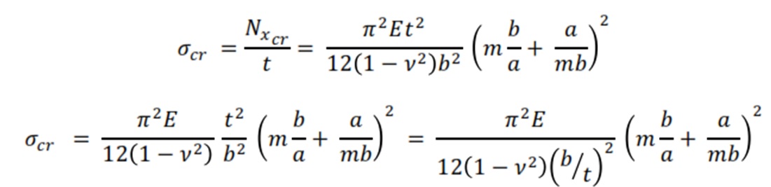
Simplifying the equation by introducing the expression for the buckling coefficient: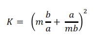 The final expression for the critical buckling stress looks as follows:
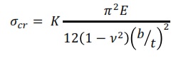 For analysis of a simply supported plate including material nonlinearity such as plasticity, the equation can be written as follow:
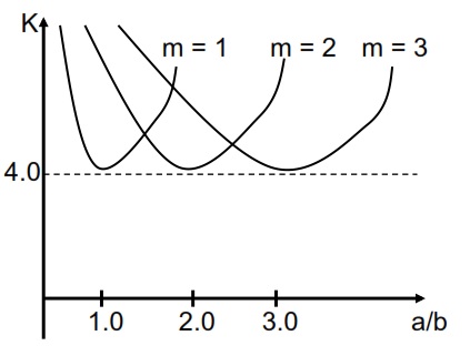
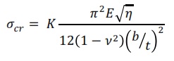 Where η = Et/E is reduction factor, with Et and E are the tangent modulus and the Young’s modulus respectively. The buckling coefficient varies with the aspect ratio and also with the number of half waves over the length of the plate, m, which can be seen in Figure below. Plates that are loaded in uniaxial compression have different values of the buckling coefficient if for example compared against a plate subjected to in-plane shear load.
The buckling coefficient can be different according to the type of loading, if it is shear or compression, and if the plate is curved or flat (see Bhrun or Niu book).
Buckling with Finite Element approach
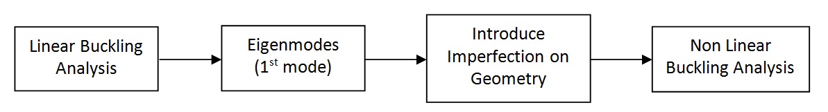
The Finite Elemet buckling analysis can be carried out by three steps: linear analysis, non linear analysis, post buckling. The linear buckling analysis as an eigenvalue problem whose smallest root defines the smallest level of external load for which there is bifurcation i.e. where two equilibrium paths intersect. The eigenvalue problem looks like the following:
![]()
where [K] is the stiffness matrix, λcr is the eigenvalue, [Kσ]ref is the stress stiffness matrix and {δu} is the eigenvector. The magnitude of the eigenvector is normalized in a linear buckling analysis problem meaning that it defines the shape of the eigenmode but not the amplitude. The linear buckling analysis consists of two subcases. In the first subcase the load is applied and in the second subcase, the eigenpairs are calculated using an extraction method e.g. the Lanczos method or the Subspace method. The Subspace iteration method is very robust but the speed is dependent on the starting subspace while the Lanczos method is very effective in the case when solving for many eigenpairs.
Generally, the buckling load obtained from a linear buckling analysis is higher than the true buckling load of a structure. The reason is that there are no imperfections included in a linear
buckling analysis, which are present when doing experimental testing. The nonlinear buckling analysis is a simulation procedure that allows for large deformationsand geometrical and/or material nonlinearities. This type of analysis is the second step after alinear buckling analysis approach.
There are three main types of nonlinearities:
- Material nonlinearity, in which material properties are functions of stress or strain.
- Contact nonlinearity, in which gaps between parts can open/close or the contact area between adjacent parts change.
- Geometric nonlinearity, in which deformations are large enough to make the small displacement assumption invalid.
In nonlinear analysis, the stiffness matrix [K] and/or the load vector {f } in the structural equations, [K] {u} = {f } , become functions of the displacements, {u}. This makes it no longer possible to solve the systems of equations directly for the displacements by inverting the stiffness matrix. Consequently, a tangent stiffness matrix, [K]t , is created, which includes both the effect of changing geometry as well as stiffening due to stress. The procedure then becomes to solve [K]t {Δu}={Δf } by use of an incremental scheme, e.g. the NewtonRaphson method (see figure below).
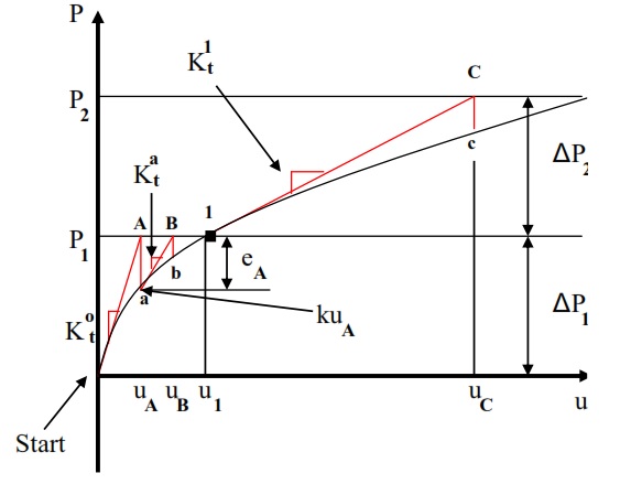
The Newton-Raphson method is the most rapidly convergent process and has a quadratic convergence rate and is also the most commonly implemented solution scheme in commercial FE software. When performing nonlinear buckling analysis of plates, the usually used geometrical models in the simulations are perfectly flat plates, where all nodes are in the same plane.
Consequently, the plates will not buckle without putting in some small imperfection in the structure. In reality, there are no plates that are produced perfectly flat without any defects and this has to be taken into account when creating FE models of this nature.
There are several ways of modeling imperfections e.g. sometimes a small out of plane force or translation of some nodes in the normal direction of the plate is sufficient in order to excite the first eigenmode. The most common and structured way to model imperfections is to use the pattern for the first eigenmode (under the assumption that this is the true shape of the buckling mode), obtained from the linear buckling analysis. There are several ways of modeling imperfections e.g. sometimes a small out of plane force or translation of some nodes in the normal direction of the plate is sufficient in order to excite the first eigenmode. The most common and structured way to model imperfections is to use the pattern for the first eigenmode (under the assumption that this is the true shape of the buckling mode), obtained from the linear buckling analysis. The imperfections have the following form in Abaqus (Abaqus Version 6.11, 2011):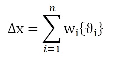 where ∆x is the magnitude of the imperfection, {Øi} is the shape of the eigenmode and wi is the amplitude or scaling factor.. MSC Nastran uses the same principle as Abaqus, but the way of applying the imperfection on to the geometry differs between the two FE solvers. In Abaqus, the keyword *IMPERFECTION is available and makes it possible to automatically chose, scale and apply the imperfection to every node by editing the input file while in MSC Nastran, this must be done manually using its pre-processor.
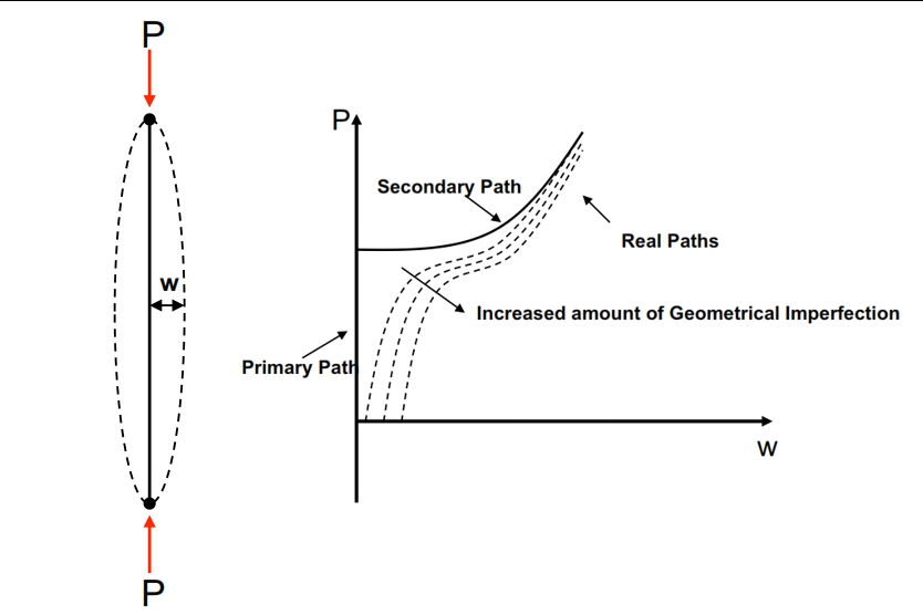
A major problem in nonlinear buckling analysis is to quantify and motivate the amount of imperfection that has to be included in the analysis. For this aim an imperfection sensitivity analysis has to be carried out. In the figure below is depicted the load versus out of plane deflection paths. it is possible to see the effect of imperfections in contrast to an ideal buckling path; including imperfections reduces the buckling load of a structure (the secondary path has no imperfections).
Postbuckling
It can be of interest to verify if the structure continues to carry the load after it has reached its critical limit or if it looses all its stiffness and collapses.
For the postbuckling study is used the Riks iteration method, it is a variant of the Arc Length method. Unlike the Newton-Raphson method, this method use an extra constraint and allows the solver to reach the convergence with lower applied load and find the equilibrium. This property of the Riks method makes it possible to trace the behavior after a limit point is reached, even though that the stiffness matrix is not positive definite. The Newton method can also work as a solution scheme when doing postbuckling analysis but only with the requirement that the postbuckling path is stable. This is hard to know in advance, so therefore the Riks method is recommended for this kind of analysis because it is valid for both stable and unstable behavior of the postbuckling paths. According to Abaqus manual (LINK), the loading during a step in the Riks solution scheme is always proportional to the current load magnitude:
![]()
Where Po is the buckling load (the value where the instability initiates), Pref is the reference load, and Г is the Load Proportionality Factor (LPF).
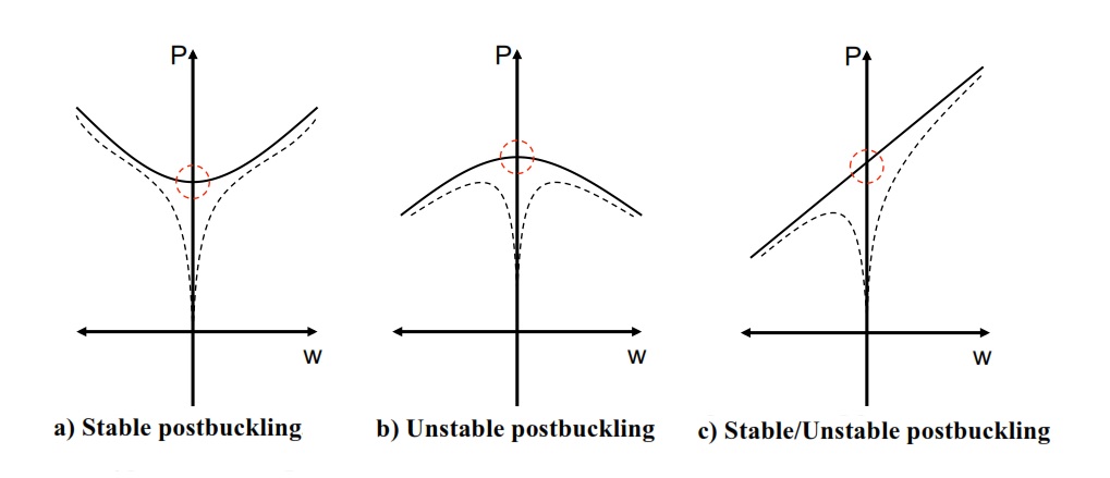
Postbuckling can be divided into two different types. The first type is called stable postbuckling and the second is called unstable postbuckling. The characteristic of stable postbuckling behavior is when the structure continues to carry the load that it is subjected and keep its stiffness (having a positive definite stiffness matrix,see figure).
The definition of unstable postbuckling is when the structure loses its stiffness and is no more able to carry the same amount of load. This often leads to that the structure starts to undergo very large geometrical changes for decreased or unchanged loading, (see Figure, case b).
NON LINEAR BUCKLING – FEM ANALYSIS WITH NASTRAN
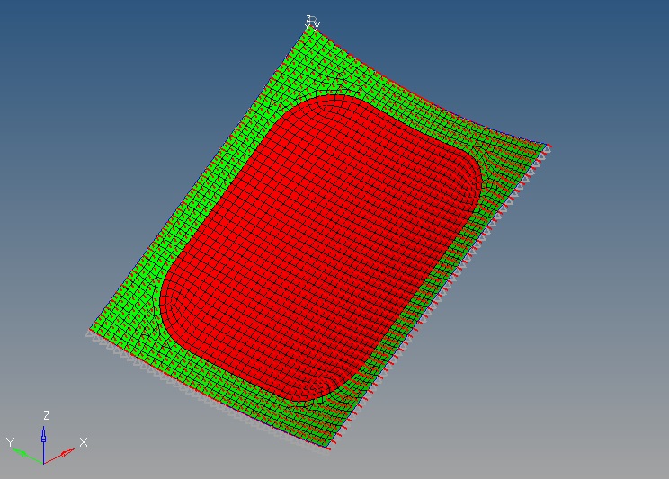
In this example is considered a plate loading with pressure and displacement along the edges (see figure below; Hypermesh and Hyperview are used for post and pre-processing).
Here is reported an exemple of Nastran run with SOL106 for the buckling. The nonlinear procedure follows a different numerical procedure. Therefore, it could provide a means for validation of linear solutions (see the post on linear buckling: Link). The Nastran file is shown below and can be downloaded.
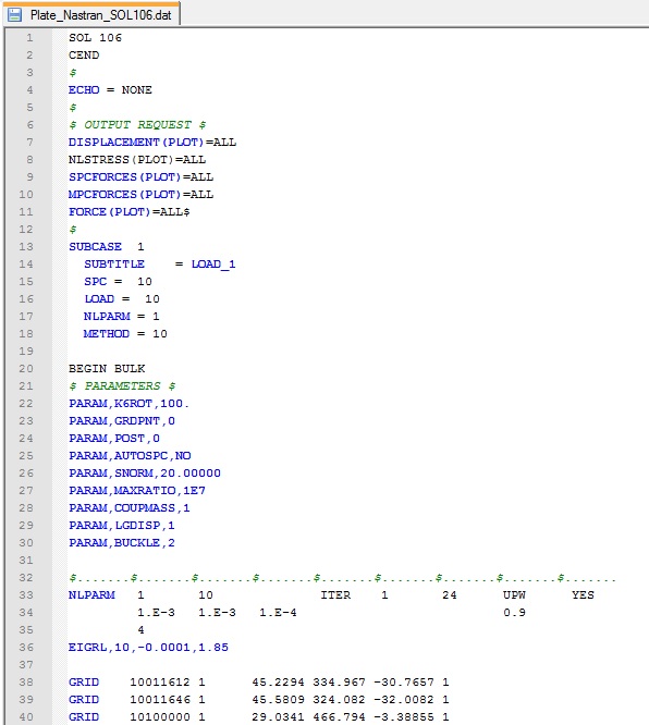
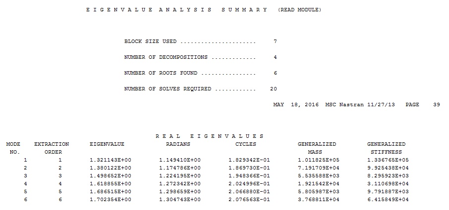
Some explanation about the setting of NLPARM use to perform the SOL106 is reported in this post. The parameters METHOD and EIGRL are menthioned in this post: Non Linear Analysis SOL 106. The parameter BUCKLE is set to 2, and thus it requests buckling in a SOL 106 cold start run. BUCKLE=1 requests a nonlinear buckling analysis in a restart run of SOLs 106 or 153. See the MSC Nastran Handbook for Nonlinear Analysis. Once the run is performed, looking the F06 file, the lower eigenvalue is equal to 1. 321143, so no buckling occurs (see figure below).
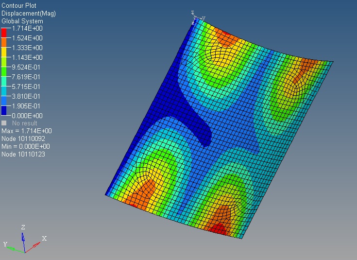
Below are plotted the results by Hyperview post-preocessing (in the second picture are plotted the deformations).
NOTE for COUPMASS parameter – There are two strategies in the finite element analysis of dynamic problems related to natural frequency determination: the consistent / coupled mass matrix and the lumped mass matrix. The coupled mass matrix is more accurate, but it has an higher computational cost with respect the lumped mass matrix method.
REFERENCE:
The content of this post has been extracted partially from “Linear and Nonlinear Buckling Analyses of Plates using the Finite Element Method”, Mert Muameleci, June 2014 (see http://www.solidmechanics.iei.liu.se/Publications/Master_theses/MasterTheses/14-01954MertMuameleciRapport.pdf)
Non Linear Buckling calculated with an alternative method
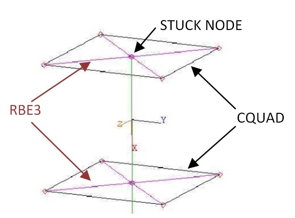
When the FEM model has a particular modellization, like a joint modeled with RBE3 and Stuck node (see figure below), the Buckling analysis could be not performed, since you will get a fatal error.
In this case the analysis can be performed by using the Nastran SOL106 as first step, and then by checking the stress on the buckled part in the direction of compression load (you can create .rpt files by Patran) for each load increment in order to understand at which load level occur the onset of Buckling. To obtain each load increment by Nastran SOL 106, it is necessary to set-up properly the NLPARM card by “YES” in the related field (see the figure below):

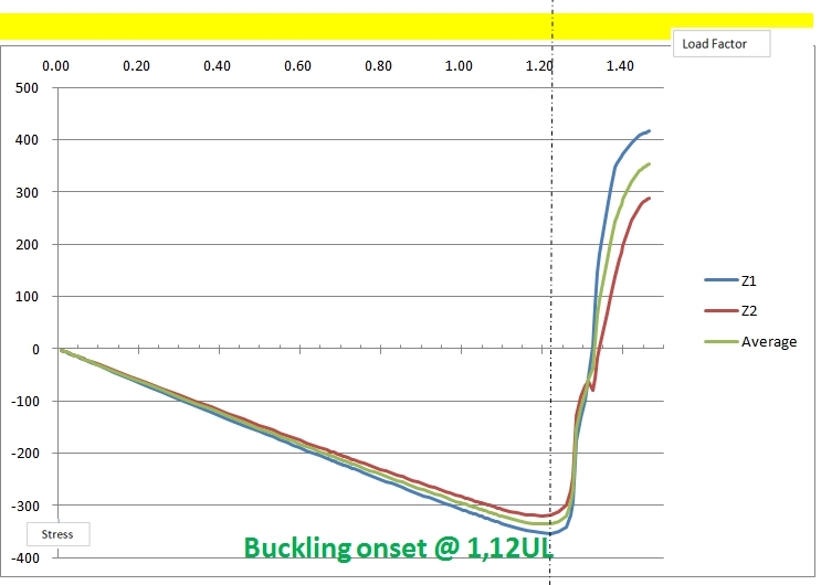
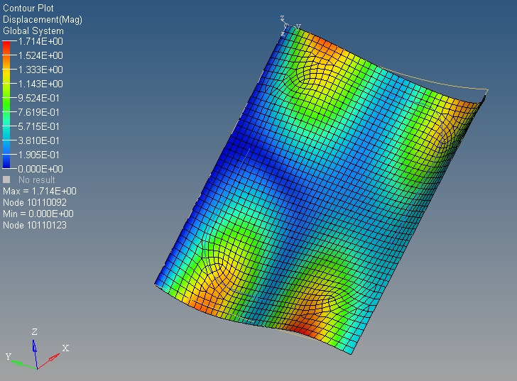
After the run of Nastran, it is necessary to identify the critical zone for buckling, by for exemple evaluating the displacements, considering the zone subjected mainly to compression where occur widest displacement out of plane, otherwise to run a linear buckling before in order to detect preliminarly the critical areas. As exemple, Below is shown the stress in X direction for a Beam at Z1 and Z2 location.
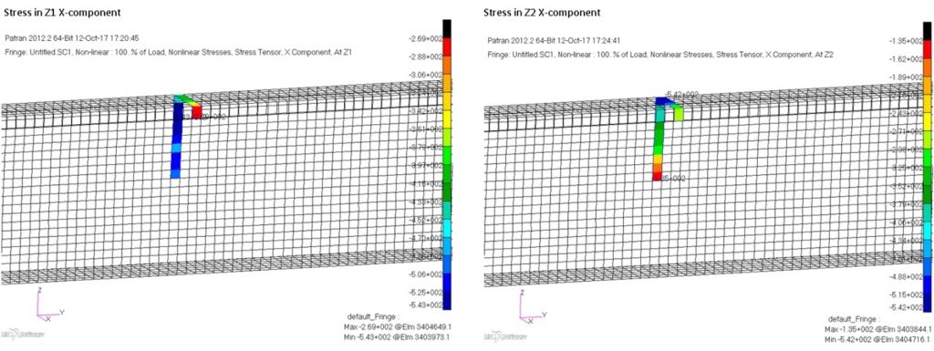
Then for each CQUAD element, like in the exemple above, can be created a curve by microsoft Excel with the load increment as abscissa, and the stress in x-direction on the vertical axis. The load factor corresponding to the maximum stress is the critical level where occurs the onset of buckling (in this case for the Element 3404770 is 1.22).