Linear Gap
The linear GAP is the simpliest contact form used in Nastran simulations. Linear GAP can solve a large class of problems like hole bearing, heel-toe interaction, fitting contacts. Linear, therefore does not include frition, large displacements, and material non-linearity. CGAP contact elements node-to-node defined in the FEM environment runs in both linear static (SOL101) and nonlinear analysis (SOL106).
The linear gaps provide for simple contact, (compressive) forces only. MPC’s are used to define the gaps. The displacements and mpc-forces are used to determine if each gap is “welded” or “free”:
- Displacement criteria: no penetration (MPC displacement >=0)
- MPCFORCE criteria: compressive force only (MPCforce <=0)
The solution converges when there is no penetration of MPCs (i.e. gap deflection >=0.0) and there are no tensile forces. An iterative procedure (CDITER – Constrained Displacement Iterative technique) is used to solve the model based on displacements/mpcforces. Below is depicted an example where the CGAP is modelled:
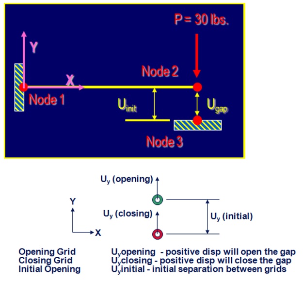
The equation for the gap displacement can be written as:
Uygap = Uyopening – Uyclosing + Uyinitial
Rearranging in MPC format and setting Uyclosing as the dependant (first) term:
Uyclosing – Uyopening + Uygap – Uyinitial = 0
The Nastran comands to use for linear gap are basically the following:
- SPOINT (Scalar Point Definition) is used to define the Ugap and Uinit :
SPOINT 55 155
- The SUPORT entry specifies reference degrees-of-freedom for rigid body motion, it puts SPOINT 55 (Ugap) in the R-set for iteration:
SUPORT 55 0
- SPC (Selects a single-point constraint set to be applied) defines initial gap opening =.05 (Uinit):
SPC 101106 155 0 .05
- MPC Entry: (Eq. of motion: Uy3 – Uy2 + Ugap – Uinit = 0)
$ SID G1 C1 A1 G2 C2 A2
MPC 101106 3 2 1.0 2 2 -1.0
$ G3 C3 A3 G4 C4 A4
55 0 1.0 155 0 -1.0
Related MSC/NASTRAN Bulk Data entries are:
- PARAM, CDITER (integer) maximum number of iterations to determine open/closed
- PARAM, CDPRT (yes/no) print iteration history of constraint violations
- PARAM, CDPCH(yes/no) punches DMIG,CDSHUT entries for final solutions
- DMIG, CDSHUT Input vector of initial open/closed state of gaps (default=all closed)
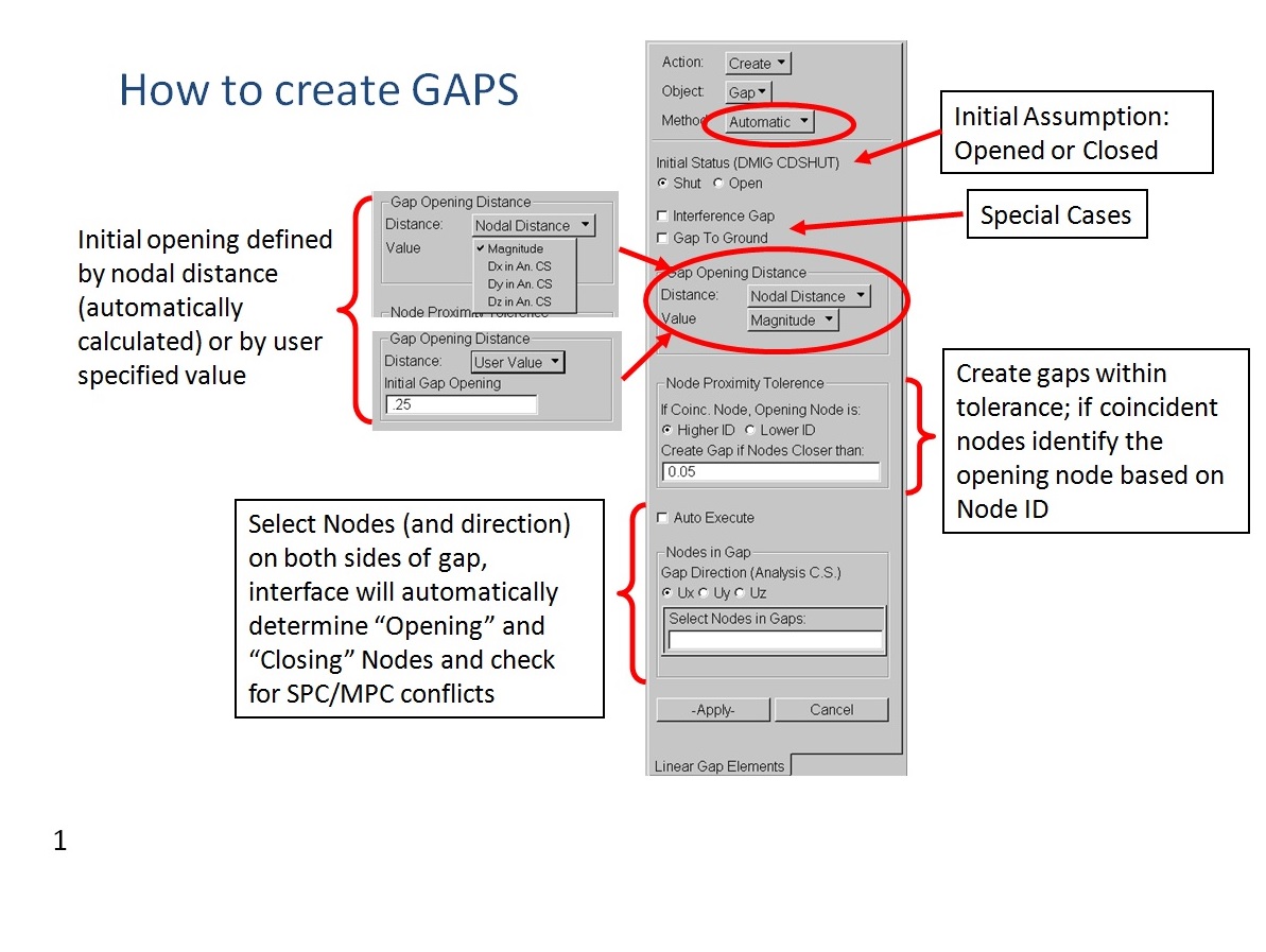
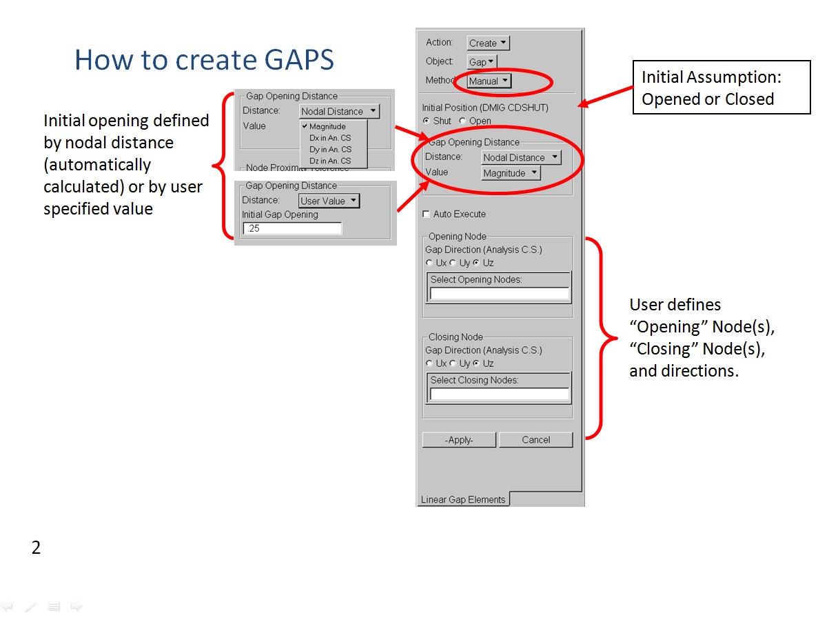
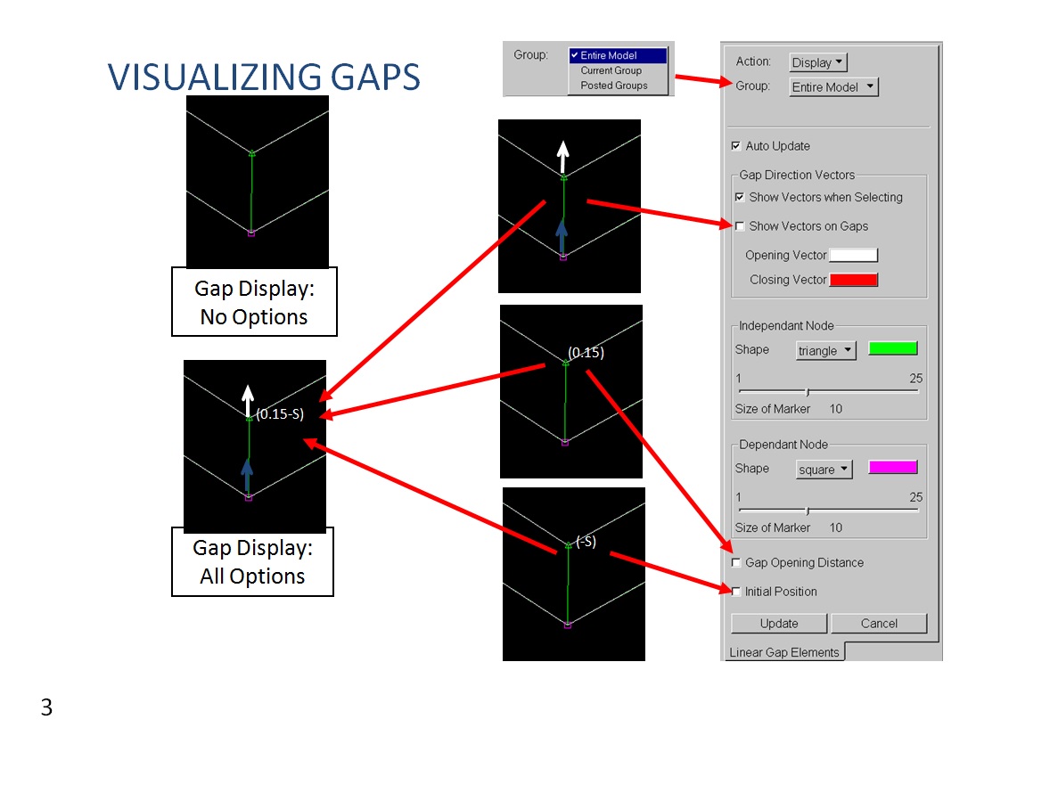
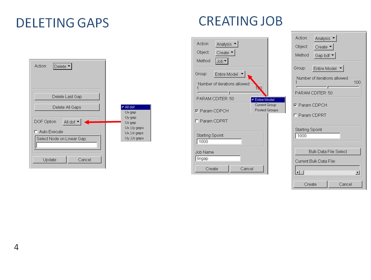
Below are shown some slide extracted from “Linear Gap New Capability Seminar“ (October 2001) where is illustrated how to create, verify and delete the CGAP elements:

Here you can download a GAP Nastran tutorial ==> exercise_05_gap_elements
Groud-Gap Example
This method is easy and relatively quick. As exemple of ground gap (analysis of a Fitting bracket) contact simulation is repoted hereafter. The model considered is made up by TET elements and RBE2s. The boundary conditions are illustradeted in the picture below:
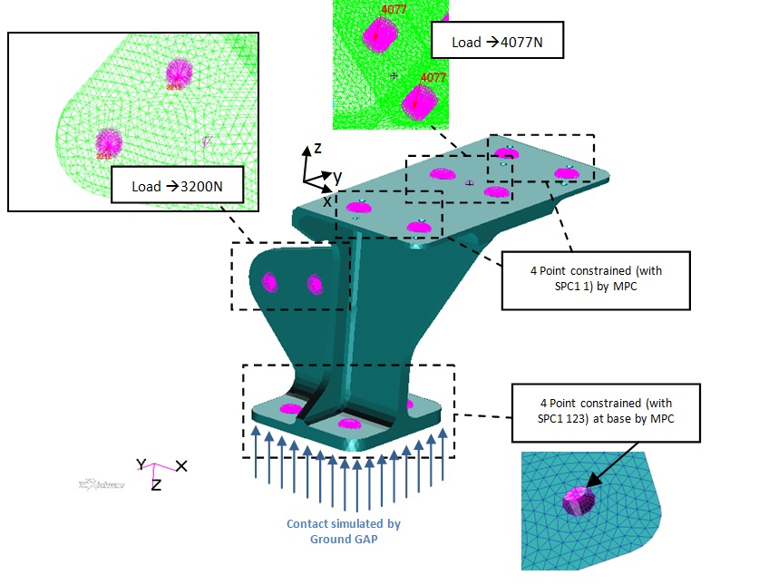
The nodes use as coordinate system reference that one with Z axis up-towards as depicted in the figure above.
To avoid “fatal” Nastran error the nodes attached directly to the RBE2s are deselected in Patran, excluding the the attached Tet elements as well (see pictures below).

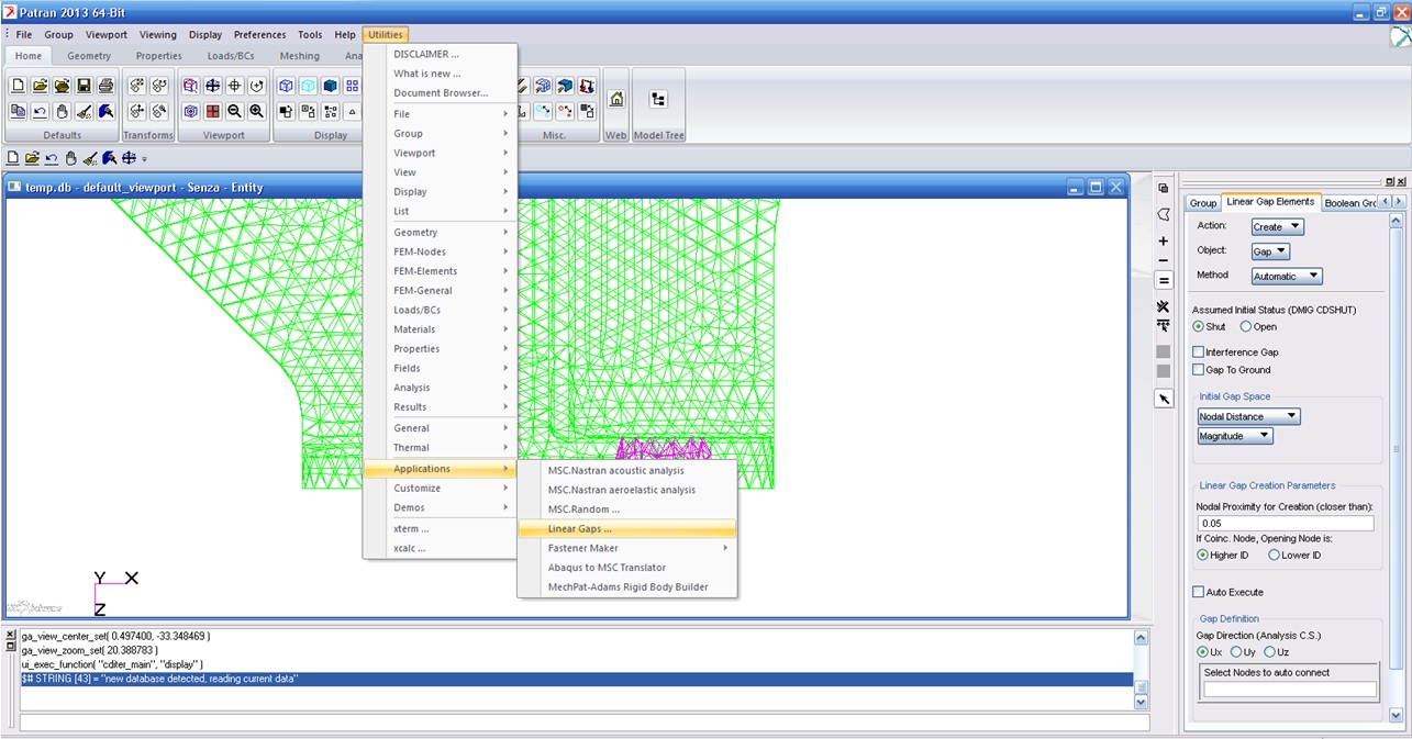
In Patran (MSC Patran 2013) the Groun GAP is created by selecting Utilities > Applications > Linear Gaps…
Then select the bottom nodes with specific option shown in the pic below:

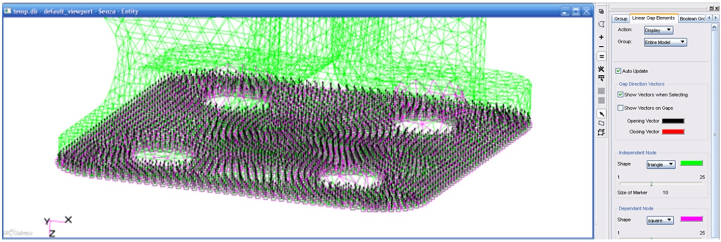
To verify the correctness of Ground GAP direction select Display and then Update in Linear Gap Elements section with the default setting as shown below:
The last step is to create GAP-data file: Utilities > Applications > Linear Gaps… > Analysis. Once you choise a name, click on Create. The file create has to be linke to the main BDF file

Here is available the files relate to the exemple illustrated above -> gap_files
Here you can download ppt file of Solid-to-Soli contact -> ws02_solid_to_solid_contact
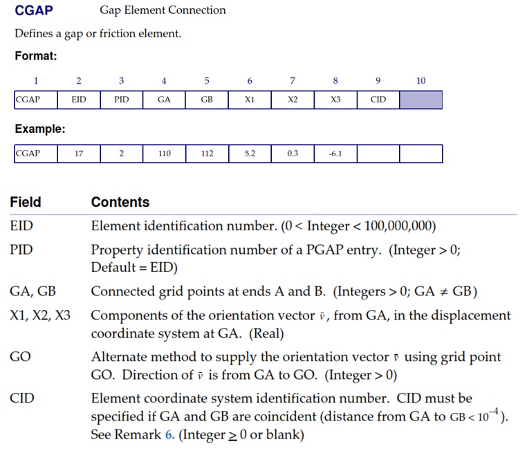
OBSERVATION – CGAP ORIENTATION
A common mistake with GAP elements is the specification of the orientation vector. The orientation vector is used to specify the orientation of the X-Y plane of the gap (like the BAR or BEAM elements) NOT the gap axial direction. The axial direction of the gap element is determined from the separation of the GRID points that define its connectivity, unless a coordinate system is defined in field 9. In this case, note that the axial direction of the gap is aligned with the T1 direction of that coordinate system, whether the grid points are coincident or not, and the X-Y plane is aligned with the T1-T2 direction of the coordinate system. If the GRID points are coincident (which is not recommended because it can cause confusion) then the gap axial direction must be specified using a coordinate system in field 9 of the CGAP card.
Limitations of Linear GAP:
- – No large displacements
- – No friction
- – No material nonlinearity
Advantages of Linear GAP:
- – Works with large models
- – Reduces the complexities inherent with SOL 106 (gap stiffness, convergence, etc.)
Non Linear Gap
Linear, therefore includes frition, large displacements, and material non-linearity. Below is reported a tutorial for contact with GAP using SOL106:
DownloadèNon-Linear Gap Elements
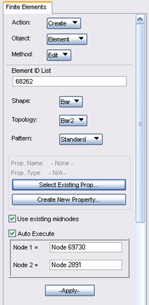
First, create an unidimensional element (BAR element) by selecting two points as shown in the figure below:
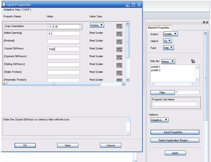
Then has to be create the GAP properties to assign at BAR created before (see the figure below for the setting by MSC Patran). The GAP as properties has an initial opening value, and closed stiffness, and it is also possible to introduce Static/Kinematic Friction even if is rarely used.
PGAP – gap element property
Below is shown the MSC/Nastran car of PGAP:
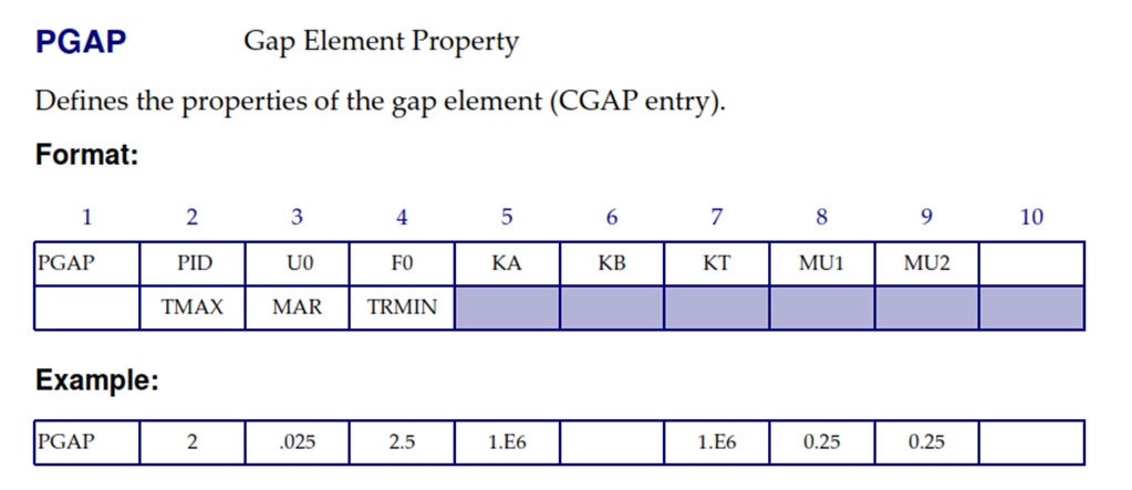
The CGAP element in MSC/NASTRAN uses the penalty method with three variants. The non-adaptive variant (TMAX=-1.0), the penalty values (KA Axial stiffness for the closed gap) remain the same throughout the analysis and there is no gap-induced stiffness update, gap-induced bisection, and sub-incremental process. In the second variant (TMAX=0.0, default value if the field is left blank) enalty values will not be adjusted, but other adaptive features will be active (i.e., the gap-induced stiffness update, gap-induced bisection, and subincremental process). The third variant (TMAX>0) is fully adaptive with all the features previously mentioned. There are certain problems which can be solved effectively with the non-adaptive gap. For instance, attached parts where all gaps are initially “overclosed” and unless plasticity is simulated, the stiffness of the surrounding structure does not change. Moreover since there is no adaptivity associated with the element, it is relatively inexpensive in terms of solution time. In the more general class of problems, however, the ability of the gap element to update its stiffness according to the changes in surrounding stiffness provides an economic solution to the non-linear problem. Below are reporte in detail the explanation of each single field.
U0: Initial gap opening, the GRIDs that define the CGAP connectivity are not used to define the initial gap open status and their separation is immaterial. The value of U0 is used to define any initial open distance of the gap, or indeed any interference or overclosure.
F0: Preload, commonly It is recommended to leave this field blank.
KA: Axial stiffness for the closed gap (when Ua – Ub > U0); to determine an initial value for KA, (because the value can be automatically modified during solution by selecting a positive value for TMAX), it is first necessary to examine the structure to which the gap element is attached. If the structure either side of the gap element is relatively stiff and only small deflections are expected in the axial direction, then a value of Young’s modulus (of the least stiff material attached to the gap) multiplied for 1000 times can be used. This is the faster way to determine a relatively quick, but approximate, suitable value of KA. Alternatively, if the structure attached to the gap element is relatively flexible, another method more that provides a better starting value for KA is to use a linear static analysis. The linear static (SOL 101) analysis should be performed prior to any non-linear analysis to determine the numerical conditioning and validity of the model. Apply a unit load, using the FORCE card, to each of the GRIDs either side of the gap elements in the axial direction of the gaps. Recover the displacements of the GRIDs of the gap elements in the gap axial direction. Divide the recovered displacement with the unit load and multiply this value by 1000 and round to the nearest order of magnitude to determine the value for KA.
KB: Axial stiffness for the open gap; this should be left at the default of 10^-14 * KA unless special gap properties are required. But the use of this parameter, with a small value of KB, provides a method of dealing with structures which may only be connected by CGAP elements, and are otherwise unconstrained. This would lead to singularities with one or both of the structures wih rigid body motion.
KT: Transverse stiffness when the gap is closed. The default value of MU1 * KA (Default) may not be appropriate if high or low values of MU1 are used. It is recommended that KT≥ 0.1*KA
MU1: Coefficient of static friction for the adaptive gap element or coefficient of friction in the y transverse direction for the nonadaptive gap element. Values for MU1 can vary between 0.0 for no friction (Default), and greater than 1.0 for non-Newtonian contact such as rubber tyres on tarmac. Typical values, like 0.15 for dry, clean steel on steel can be obtained from Kempes Engineering Handbook.
MU2: Coefficient of kinetic friction for the adaptive gap element or coefficient of friction in the z transverse direction for the nonadaptive gap element. Estimating values for sliding friction are more difficult than static friction, and could be necessary to obtain an appropriate value by tests.
TMAX: Maximum allowable penetration used in the adjustment of penalty values. If set to a negative value, the gap element has no adaptivity and retains the specified penalty values throughout the analysis. If TMAX is set to 0.0 (the default), the gap-induced stiffness update, gap-induced bisection, and sub-incremental process are enabled, but the penalty values remain unchanged. If TMAX is set to a small positive value, this has all the features of the gap when TMAX=0.0, and also enables the adaptive penalty capability where the penalty values are adjusted according to changes in the stiffness of the surrounding structure. The recommended allowable penetration TMAX is about 10% of the element thickness for plates or the equivalent thickness for other elements that are connected to the gap. If the structure is a massive solid, then the ideal value of TMAX is two or three orders of magnitude less than the elastic deformation of the solid. This is not always easy to estimate, so a value of 1 * 10^-4 of the characteristic length of the model can be used. TMAX is too small, the solution will frantically try to adjust the penalty values to update the stiffnesses. If TMAX is too large; no update will occur and convergence may be elusive.
MAR: Maximum allowable adjustment ratio for adaptive penalty values KA and KT. This sets the maximum allowable adjustment ratio for the penalty values and must be in the range 1.0 to 10^6. The upper and lower bounds of the adjusted penalty values are K/MAR and K*MAR, where K is KA or KT.
TRMIN: This is used only for the penalty value adjustment, and it sets the lower bound for the allowable penetration and is a fraction of TMAX. It must be in the range 0.0 to 1.0. Penalty values are decreased if the penetration is less than the minimum allowable penetration which is calculated from TRMIN * TMAX.
[smartslider3 slider=”2″]
[smartslider3 slider=”2″]