[kofi]
[paypal-donation]
Miner’s rule is probably the simplest cumulative damage model. It states that if there are k different stress levels (with linear damage hypothesis) and the average number of cycles to failure at the ith stress, Si, is Ni, then the damage fraction, C, is:
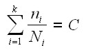
where:
– ni is the number of cycles accumulated at stress Si.
– C is the fraction of life consumed by exposure to the cycles at the different stress levels.
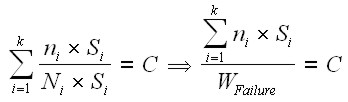
In general, when the damage fraction reaches 1, failure occurs. The above equation can be thought of as assessing the proportion of life consumed at each stress level and then adding the proportions for all the levels together. Often an index for quantifying the damage is defined as the product of stress and the number of cycles operated under this stress, which is:
![]()
Assuming that the critical damage is the same across all the stress levels, then:
![]()
For example, let’s say WFailure=50 for a component. So the component will fail after 10 cycles at a stress level of 5, or after 25 cycles to fail at a stress level of 2, and so on. Using Eqn. (2) as the critical value of damage that will result in failure, Eqn. (1) becomes:
C represents the proportion of the cumulative damage to the critical value.
Example:
A part is subjected to a fatigue environment where 10% of its life is spent at an alternating stress level, σ1, 30% is spent at a level σ2, and 60% at a level σ3. How many cycles, n, can the part undergo before failure? If, from the S-N diagram for this material the number of cycles to failure at σi is Ni (i =1,2,3), then from the Palmgren-Miner rule failure occurs when:
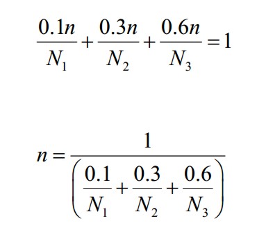
Above is shown the solution for n cycles given.
Note:
1. “High-low” fatigue tests where testing occurs sequentially at two stress levels ( σ1 ,σ2) where σ1 >σ2 generally shows that failure occurs when
where C normally is < 1, i.e the Palmgren-Miner rule is non-conservative for these tests. For “low-high” tests, c values are typically > 1.
2. For tests with random loading histories at several stress levels, correlation with the Palmgren-Miner rule is generally very good.
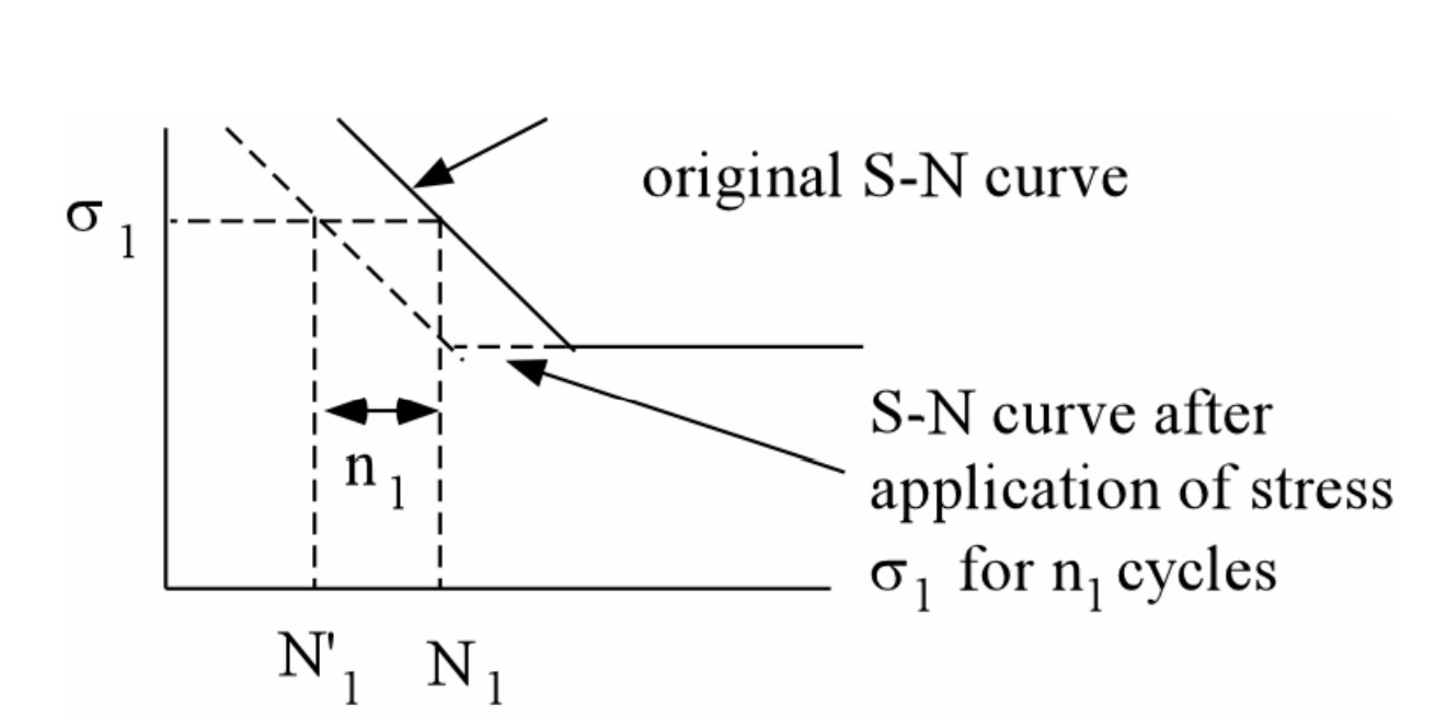
3. The Palmgren-Miner rule can be interpreted graphically as a “shift” of the S-N curve. For example, if N1 cycles are applied at stress level σ1 (where the life is N1 cycles), the S-N curve is shifted so that goes through a new life value, N’1.
Limitations
A major limitation of the Palmgren-Miner rule is that it does not consider sequence effects, i.e. the order of the loading makes no difference in this rule. Sequence effects are definitely observed in many cases. A second limitation is that the Palmgren-Miner rule says that the damage accumulation is independent of stress level. This can be seen from the modified S-N diagram above where the entire curve is shifted the same amount, regardless of stress amplitude.
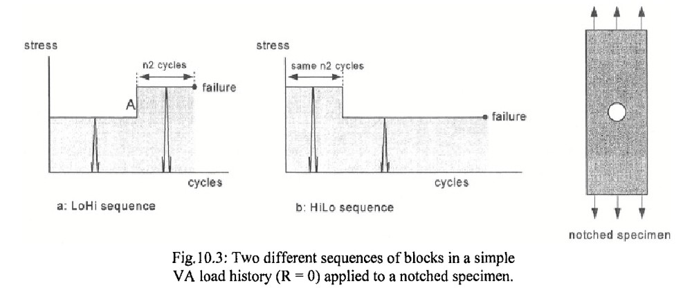
Limitation: Effect of Notch Plasticity (“Fatigue of Structures and Materials – Jaap Schijve”)


Crak length at failure:
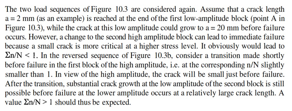
(Source: “Fatigue of Structures and Materials – Jaap Schijve”)
if you have appreciated this post, please click on the banner below, thanks.
[smartslider3 slider=”2″]
[kofi]
[paypal-donation]
Pingback: Random Vibration Analysis – Nastran SOL 111 | Aerospace Engineering