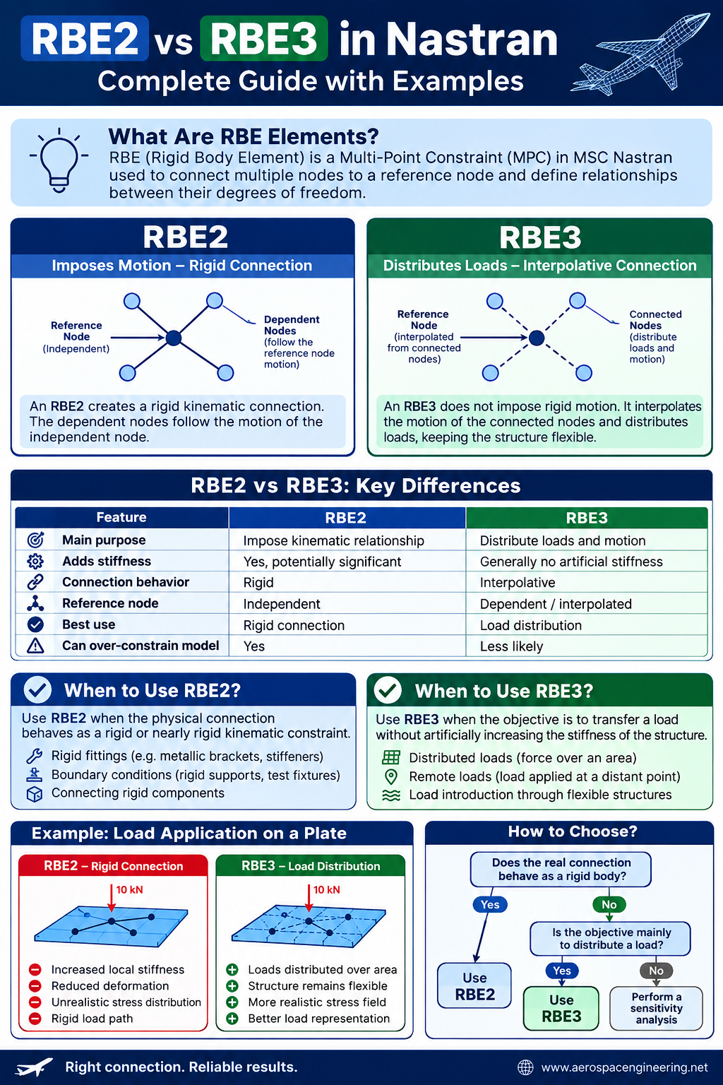
RBE2 vs RBE3 in Nastran: Complete Guide with Examples
Finite Element Analysis is only as good as the way loads, constraints, and connections are represented. In MSC Nastran, two of the most widely used elements for connecting parts of a finite element model are RBE2 and RBE3.
At first glance, they may appear similar. Both connect multiple nodes to a reference node. However, their mechanical behavior is fundamentally different.
Using the wrong one can:
- artificially increase the stiffness of a structure;
- create unrealistic load paths;
- generate misleading stress concentrations;
- distribute loads incorrectly;
- affect modal and buckling results.
This guide explains the difference between RBE2 and RBE3, when to use each one, and the most common modeling mistakes.
What Is an RBE Element?
RBE stands for Rigid Body Element. In Nastran, RBE elements are Multi-Point Constraints (MPCs) used to define relationships between degrees of freedom of different nodes.
The most common rigid elements are:
- RBE2
- RBE3
Although both involve a reference node and several connected nodes, they solve completely different modeling problems.
The simplest way to remember the difference is:
RBE2 imposes motion. RBE3 distributes load.
That single concept is the foundation for understanding when each element should be used.
1. What Is an RBE2?
An RBE2 element creates a rigid kinematic connection between one independent node and one or more dependent nodes.
The motion of the dependent nodes is constrained by the motion of the independent node.
In simplified form:
Dependent node displacement = motion imposed by the independent node
If the independent node translates, the connected nodes follow that motion.
If the independent node rotates, the connected nodes move according to a rigid-body relationship.
This means that an RBE2 introduces a rigid connection between the selected degrees of freedom.
Basic RBE2 Configuration
An RBE2 typically contains:
- one independent node;
- multiple dependent nodes;
- selected degrees of freedom.
For example, an RBE2 may connect a central reference node to the nodes around a circular hole.
If all six degrees of freedom are selected:
- translations: 1, 2, 3;
- rotations: 4, 5, 6.
the connected region behaves as if it were connected to a rigid structure.
RBE2 Example: Applying a Load Through a Bolt Hole
Imagine a plate with a circular hole.
You want to apply a force through the center of the hole.
A simple model could look like this:
           o   o
        o         o

            ●
         Reference
            Node

        o         o
           o   o
The nodes around the hole are connected to the central reference node using an RBE2.
A force can then be applied at the central node.
The RBE2 transfers the motion and load through the connected nodes.
This can be useful when the real structure is connected to a component that is significantly stiffer than the surrounding structure.
For example:
- rigid brackets;
- stiff fittings;
- idealized joints;
- actuators;
- test fixtures.
However, there is an important risk.
The RBE2 may make the surrounding structure artificially stiff.
2. What Is an RBE3?
An RBE3 element does not create a rigid connection between the reference node and the connected nodes.
Instead, it creates an interpolation relationship.
The motion of the reference node is calculated as a weighted average of the motion of the connected nodes.
Conceptually:
Reference Node Motion
          ↓
Calculated from
          ↓
Weighted Motion of Connected Nodes
This means that an RBE3 generally distributes loads without imposing significant artificial stiffness on the connected structure.
That is why RBE3 elements are extremely useful when loads must be distributed over an area.
The Most Important Concept
With an RBE3:
The connected structure remains flexible.
The RBE3 transfers forces and moments according to the specified interpolation and weighting.
Unlike an RBE2, it does not force the connected nodes to behave like part of a rigid body.
3. RBE2 vs RBE3: The Fundamental Difference
The difference can be summarized as follows:
| Feature | RBE2 | RBE3 |
|---|---|---|
| Main purpose | Impose kinematic relationship | Distribute loads and motion |
| Adds stiffness | Yes, potentially significant | Generally no artificial stiffness |
| Connection behavior | Rigid | Interpolative |
| Reference node | Independent | Dependent/interpolated |
| Best use | Rigid connection | Load distribution |
| Can over-constrain model | Yes | Less likely |
| Suitable for distributed loads | Sometimes | Excellent |
| Suitable for rigid fittings | Excellent | Usually not appropriate |
The key difference is therefore:
RBE2 controls displacement.
RBE3 calculates displacement and distributes loads.
4. Example: Applying a Force to a Circular Area
Consider a 10 kN force applied to the center of a circular plate.
There are two possible approaches.
Case A: Using an RBE2
The central node is connected to the surrounding nodes using an RBE2.
              10 kN
                ↓
                ●
             RBE2 Node
            /  |  \
          o----o----o
         /           \
        o             o
The nodes connected to the RBE2 are forced to follow the rigid-body motion of the reference node.
The result may be:
- reduced local deformation;
- increased stiffness;
- altered stress distribution;
- unrealistic load path if the actual load introduction mechanism is flexible.
The model may look perfectly stable and produce apparently reasonable stresses.
However, the physical behavior may be incorrect.
Case B: Using an RBE3
Now the same 10 kN load is applied to a reference node connected through an RBE3.
              10 kN
                ↓
                ●
             RBE3 Node
            /  |  \
          o    o    o
         /           \
        o             o
The force is distributed among the connected nodes.
The plate remains free to deform according to its actual stiffness.
The resulting stress and displacement field is generally more representative of a distributed load introduction.
For this reason, RBE3 is often the preferred choice for:
- distributed forces;
- aerodynamic loads;
- pressure load idealization;
- inertia load transfer;
- remote loads;
- actuator load introduction.
5. When Should You Use RBE2?
An RBE2 should be used when the physical connection is intended to behave as a rigid or nearly rigid kinematic constraint.
Typical applications include:
Rigid fittings
If a metallic fitting is significantly stiffer than the connected structure, an RBE2 may be an appropriate idealization.
For example:
Flexible Structure
       │
       │
   [ RBE2 ]
       │
       ●
   Reference Node
The RBE2 represents the stiff connection.
Boundary Conditions
RBE2 elements can also be used to connect a group of nodes to a reference node where boundary conditions are applied.
For example:
- test fixtures;
- rigid supports;
- simplified interfaces;
- idealized mounting points.
Care must be taken to avoid creating unrealistic stiffness.
Connecting Rigid Components
If a component is known to be much stiffer than the surrounding structure, representing the connection using an RBE2 may be computationally efficient.
However, the assumption should always be verified.
A component that appears rigid in reality may still introduce local flexibility that is important for:
- stress analysis;
- fatigue;
- vibration;
- buckling.
6. When Should You Use RBE3?
An RBE3 is usually the better choice when the objective is to transfer a load without artificially increasing the stiffness of the structure.
Typical applications include:
Distributed Loads
Suppose a force must be applied over a structural interface.
Instead of applying the entire force to one node, an RBE3 can distribute the force among multiple nodes.
This reduces unrealistic local stress concentrations.
Remote Loads
A remote force may be defined at a reference point located away from the structure.
For example:
      Load Application Point
              ●
              │
              │
             RBE3
          /    |    \
         o     o     o
The load is transferred to the structure while allowing the connected nodes to deform naturally.
Load Introduction Through Flexible Structures
An RBE3 is particularly useful when the actual load introduction mechanism is not perfectly rigid.
Examples include:
- aerodynamic pressure resultants;
- distributed mechanical loads;
- interfaces represented by multiple structural nodes;
- simplified connection regions.
7. The Artificial Stiffness Problem
One of the most common FEM modeling mistakes is using an RBE2 where an RBE3 should have been used.
Consider a flexible plate.
If an RBE2 connects a large group of nodes to a central node, the connected region may behave like a rigid body.
The local flexibility of the plate is reduced.
This can affect:
- displacement;
- stress distribution;
- natural frequencies;
- buckling load;
- load path.
The effect becomes particularly significant when the RBE2 connects nodes over a large area.
A large RBE2 spider can effectively create a rigid plate inside a flexible structure.
This is often physically unrealistic.
8. The “Rigid Spider” Effect
A common modeling technique is to create a spider connection.
For example:
        o       o
          \   /
            ●
          /   \
        o       o
The central node is connected to surrounding nodes.
If an RBE2 is used, the spider behaves rigidly.
If the same configuration uses an RBE3, the structure remains flexible.
This distinction is critical.
A useful rule is:
If the spider is only required to distribute a load, start by considering RBE3.
If the spider represents a genuinely rigid connection, RBE2 may be appropriate.
9. Load Distribution with RBE3 Weighting Factors
RBE3 elements can use weighting factors to control how loads are distributed among connected nodes.
For example, assume four nodes:
Node A → Weight 1
Node B → Weight 1
Node C → Weight 2
Node D → Weight 2
Nodes C and D will have a greater contribution to the interpolation.
Weighting can be useful when the load should not be distributed uniformly.
For example:
- different structural areas;
- different stiffness regions;
- asymmetric load paths;
- aerodynamic resultant locations.
However, weighting should not be used arbitrarily.
The weighting strategy should represent a physically meaningful load distribution.
10. RBE2 and RBE3 in Modal Analysis
Rigid elements can have a significant influence on modal analysis.
RBE2
An RBE2 can increase the effective stiffness of the model.
As a result, natural frequencies may increase.
The effect depends on:
- number of connected nodes;
- size of the connection;
- selected degrees of freedom;
- flexibility of the surrounding structure.
A large RBE2 in a flexible structure can significantly alter the mode shapes.
RBE3
An RBE3 generally allows the connected structure to retain its flexibility.
Therefore, it is often preferable when a load or mass must be distributed without creating an artificial rigid region.
However, the complete dynamic model must still be checked carefully.
For modal analysis, always verify:
- rigid body modes;
- connectivity;
- mass distribution;
- constraints;
- mode shapes.
11. RBE2 and RBE3 in Buckling Analysis
The choice between RBE2 and RBE3 can also affect buckling results.
Consider a thin panel subjected to compression.
If an RBE2 artificially stiffens the load introduction region, the predicted buckling load may be higher than the real value.
The model may show:
RBE2 → Increased Local Stiffness
      ↓
Higher Predicted Buckling Load
      ↓
Potentially Non-Conservative Result
Using an RBE3 may provide a more realistic load distribution while allowing the structure to deform.
For buckling analysis, always compare:
- RBE2 vs RBE3 results;
- displacement field;
- stress distribution;
- eigenvectors;
- local deformation near the connection.
A sensitivity study can reveal whether the modeling choice significantly affects the results.
12. Common Mistakes When Using RBE2
Mistake 1: Connecting Too Large an Area
A large RBE2 spider can create an unrealistic rigid zone.
Better approach
Use:
- a smaller connection area;
- RBE3 for load distribution;
- a detailed connection model;
- flexible elements.
Mistake 2: Constraining Too Many Degrees of Freedom
It is not always necessary to connect all six degrees of freedom.
For shell models, the selected DOFs should reflect the actual physical connection.
For example, connecting rotations unnecessarily may introduce unrealistic constraints.
Always ask:
Which motion is actually transferred by the real component?
Mistake 3: Ignoring the Load Path
An RBE2 may create a load path that does not exist in the real structure.
The model can transfer forces through a rigid mechanism that would actually deform significantly.
Always examine:
- where the force enters the structure;
- which components transfer the load;
- which regions are flexible;
- which interfaces are actually rigid.
13. Common Mistakes When Using RBE3
Mistake 1: Using RBE3 as a Physical Rigid Connection
An RBE3 should not be used when the objective is to enforce rigid-body motion.
If a component must move rigidly, an RBE2 or another appropriate connection method may be required.
Mistake 2: Incorrect Weighting
Weight factors can significantly affect the load distribution.
Incorrect weights may create:
- unrealistic forces;
- unexpected moments;
- asymmetric load transfer.
The weighting should be based on geometry or physical load distribution whenever possible.
Mistake 3: Ignoring Rotational Degrees of Freedom
The selected DOFs must match the modeling objective.
A poorly defined RBE3 can transfer loads in an unexpected way.
Always inspect:
- SPC forces;
- MPC forces;
- reaction forces;
- equilibrium.
14. How to Choose Between RBE2 and RBE3
Use this simple decision process.
Question 1
Does the real connection behave as a rigid body?
If yes:
→ Consider RBE2.
If no:
→ Continue.
Question 2
Is the objective mainly to distribute a load across multiple nodes?
If yes:
→ Consider RBE3.
Question 3
Would an artificial rigid zone affect the results?
If yes:
→ Prefer RBE3 or a more realistic connection model.
Question 4
Are you analyzing local stress, buckling, or modal behavior?
If yes:
→ Perform a sensitivity analysis because the choice of rigid element may significantly affect the results.
15. RBE2 vs RBE3: Practical Decision Table
| Modeling Situation | Recommended Approach |
|---|---|
| Rigid fixture | RBE2 |
| Very stiff fitting | RBE2 |
| Distributed force | RBE3 |
| Remote load | RBE3 |
| Load applied over flexible area | RBE3 |
| Idealized rigid interface | RBE2 |
| Modal analysis load distribution | Usually RBE3 |
| Buckling load introduction | Often RBE3, verify sensitivity |
| Bolt hole load introduction | Depends on joint stiffness |
| Test fixture connection | Often RBE2 |
| Flexible mechanical interface | RBE3 or detailed model |
16. A Practical Workflow for Aerospace FEM Models
Before creating an RBE element, follow this process.
Step 1: Understand the physical connection
Ask:
- Is the connection rigid?
- Is it flexible?
- Does it transmit moments?
- Does it allow rotation?
- Is the load concentrated or distributed?
Step 2: Define the modeling objective
Are you evaluating:
- global displacement?
- local stress?
- fatigue?
- buckling?
- modal response?
The required modeling fidelity may change.
Step 3: Select the connection method
Choose between:
- RBE2;
- RBE3;
- CBUSH;
- CELAS;
- MPC;
- detailed solid or shell connection.
Step 4: Verify the load path
Check:
- SPC forces;
- free body equilibrium;
- force balance;
- deformation pattern.
Step 5: Perform a sensitivity study
When results are important, compare alternative connection methods.
For example:
Model A → RBE2
Model B → RBE3
Model C → Flexible connection
Compare:
- displacement;
- stress;
- reaction forces;
- natural frequencies;
- buckling factors.
If the results change significantly, the connection modeling assumption is important and should be investigated further.
Frequently Asked Questions
Does RBE2 increase stiffness?
Yes. An RBE2 imposes rigid kinematic relationships between nodes and can significantly increase the local or global stiffness of a finite element model.
The effect depends on the geometry, connected degrees of freedom, and flexibility of the surrounding structure.
Does RBE3 add stiffness?
An RBE3 is generally used to distribute loads and interpolate motion without creating the same artificial rigid region associated with an RBE2.
However, the complete constraint system must always be checked to ensure that the model behaves as intended.
Can RBE2 and RBE3 be used together?
Yes.
In complex models, an RBE2 may represent a rigid component while an RBE3 distributes a load from another interface.
The important point is to avoid creating conflicting constraints or unrealistic load paths.
Which one is better for applying a force?
If the force must be distributed over a flexible structure, an RBE3 is usually the preferred option.
If the force is transmitted through a genuinely rigid component, an RBE2 may be more appropriate.
Is RBE2 always wrong for bolt holes?
No.
The correct choice depends on the physical joint.
A rigid bolt or fitting may justify an RBE2 approximation for some global analyses.
For local stress, bearing loads, joint flexibility, or fatigue analysis, a more detailed representation may be necessary.
Conclusion
RBE2 and RBE3 elements are among the most powerful and frequently misunderstood modeling tools in MSC Nastran.
The difference is simple but fundamental:
RBE2 imposes a rigid kinematic relationship.
RBE3 distributes loads and interpolates motion without imposing the same rigid behavior.
An RBE2 is appropriate when the physical connection is genuinely rigid or when a rigid constraint is intentionally required.
An RBE3 is generally more appropriate when a load must be distributed across a flexible structure without artificially increasing its stiffness.
The best practice is not to choose an RBE element based on habit.
Instead, start from the real physical behavior, identify the expected load path, and verify the modeling assumption through sensitivity analysis.
In aerospace structural analysis, a seemingly small modeling decision—such as choosing RBE2 instead of RBE3—can influence stress, displacement, natural frequencies, and buckling results.
For that reason, the question should never simply be:
“Which element should I use?”
The real question is:
“What physical behavior am I trying to reproduce?”
If you answer that correctly, choosing between RBE2 and RBE3 becomes much easier.
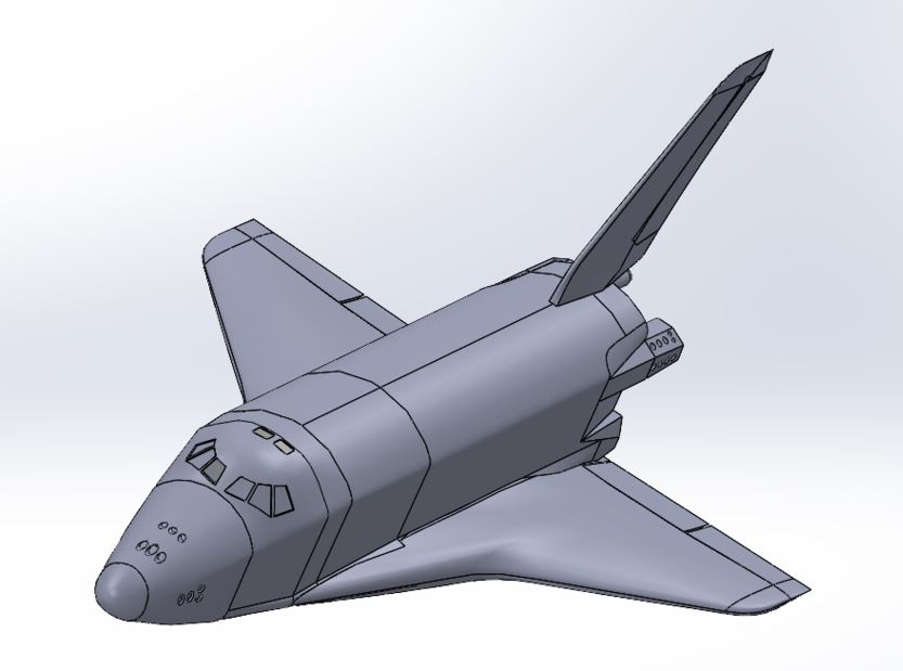
Buran – Russian Space Shuttle – 3D Model
Buran
A simple geometrical model of Soviet Space Shuttle without interior
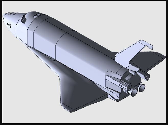

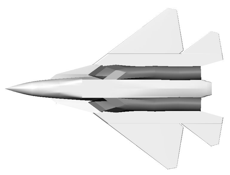
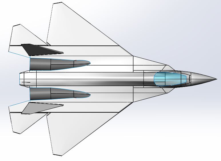
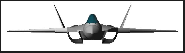
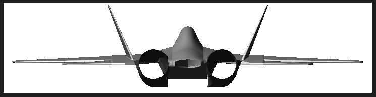
Fighter Jet 36 – 3D Model
Fighter Jet 36 – 3D Model
PAK FA from the years 2004–2005.
Surface Modeling
only for educational purpose
Details
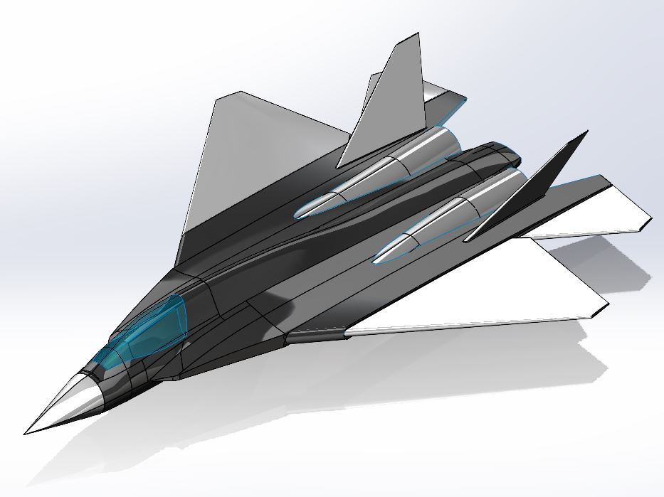
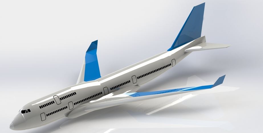
Boeing B747 – 3D Model
Boeing B747
A simplified Boeing B747 model created in SolidWorks as a single solid body.
The design captures the general shape and proportions of the world’s largest passenger aircraft — ideal for rendering, concept visualization, or aerodynamic study.
No internal details, turbines, or landing gear are included for simplicity and smooth performance.
Modeled entirely in SolidWorks
Lightweight and easy to render
Suitable for concept or educational purposes
3I/ATLAS: Between Science and Mystery
3I/ATLAS is an extrasolar interstellar object currently passing through our Solar System, and its discovery has generated enormous scientific and media attention between 2025 and 2026. Officially designated C/2025 N1 (ATLAS), it was identified on July 1, 2025, by the Chilean telescope of the Asteroid Terrestrial-impact Last Alert System (ATLAS).
The prefix 3I indicates that this is the third confirmed interstellar object detected passing through our Solar System, following ʻOumuamua (2017) and 2I/Borisov (2019).
🔭 Scientific Characteristics Based on Observational Data
🚀 Trajectory and Velocity
The orbital path of 3I/ATLAS is not a closed orbit like those of planets or typical comets in our Solar System, but hyperbolic, meaning the object will enter and exit the Solar System without being gravitationally captured.
Its orbital eccentricity is extremely high — far greater than that of any previously observed Solar System body — and the object travels at speeds of tens of kilometers per second.
A hyperbolic trajectory combined with such high velocity unequivocally indicates an origin outside the Solar System, as these parameters cannot be explained by the gravitational processes governing bodies formed around the Sun.

🧪 Chemical Composition and Activity
Spectroscopic observations, including those obtained by the James Webb Space Telescope (JWST), reveal that the object possesses a coma dominated by carbon dioxide (CO₂), with the presence of water, carbon monoxide, oxides, water ice, and icy dust.
These relative gas abundances are unusual but consistent with a primordial cosmic body formed around another stellar system during the early stages of planet formation.
Further studies also indicate the emission of hydroxyl radicals (OH), attributable to the photodissociation of water molecules under solar radiation — a clear sign of natural outgassing processes typical of comets.
🌌 X-Ray Observations
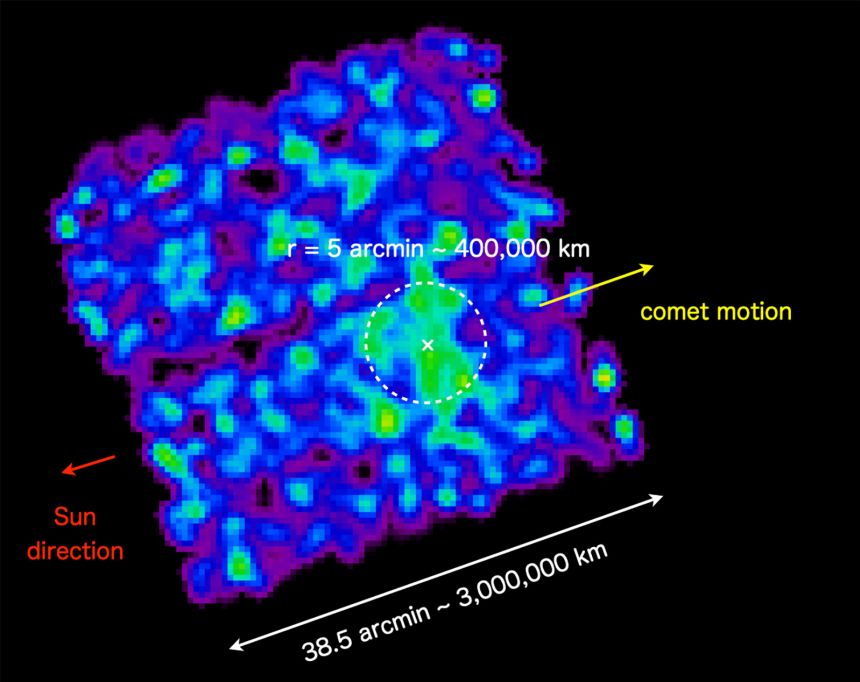
Instruments such as ESA’s XMM-Newton and Japan’s XRISM observatory detected X-ray emissions extending roughly 250,000 miles from the nucleus of 3I/ATLAS. These emissions result from the interaction between the object’s gaseous envelope and the solar wind.
Such observations help scientists better understand the physical and plasma processes that characterize interstellar objects as they pass through the Solar System.
Interstellar comet glows in new X-ray images ahead of Earth flyby | CNN
🧠 Why This Object Matters to Science
🔁 A Window into Other Stellar Systems
From compositional and dynamical studies, 3I/ATLAS may originate from a stellar system billions of years old, possibly even older than our Sun.
Analyzing its atmosphere, volatile compounds, and dust provides a rare opportunity to study the chemistry of material formed around other stars — an opportunity that may arise only once every decade or even less frequently.
🛸 Speculation and Extraterrestrial Theories
Since its discovery, 3I/ATLAS has sparked widespread speculation across the internet and in the media, often fueled by the allure of the unknown.
👽 Hypotheses of Intelligent Navigation
Some researchers, including astrophysicist Avi Loeb, have cautiously suggested — in tones less conventional than mainstream astronomy — that certain characteristics, such as apparent “pulsations” or subtle trajectory anomalies, could leave room for non-natural or technological scenarios.
These ideas are not supported by direct evidence, but rather by interpretations of incomplete data that have not yet found fully satisfactory explanations. Nevertheless, they have fueled fascinating debates among the public and within limited scientific circles.
🧩 Extreme Theories from Online Communities
In forums and social media spaces, even more imaginative narratives have emerged, including the idea that 3I/ATLAS might be an alien probe, a macroscopic quantum object, or even a vehicle of interstellar consciousness. These stories often involve sensational “leaks” or alleged anomalous behaviors that are not confirmed by official observations.
It is important to emphasize that such claims have no support within the academic community and frequently contradict well-established physical laws.
📉 The Scientific Consensus
Despite occasional speculation, the scientific community overwhelmingly agrees that 3I/ATLAS is a natural object, specifically an interstellar comet, and not a technological artifact or extraterrestrial spacecraft.
Evidence based on spectroscopy, orbital dynamics, and physical behavior consistently points to processes fully compatible with cometary physics, albeit in an object that is rare and extraordinary.
🌠 Conclusion: Between Science and Imagination
3I/ATLAS challenges our scientific understanding not because it violates the laws of physics, but because it carries direct information from another stellar system — something that may happen only once in a century.
Its passage invites us to:
-
Reconsider the diversity of cosmic objects beyond our Solar System
-
Study the chemical origins of other planetary systems, including unfamiliar molecules and dust
-
Remain open yet critical toward unconventional explanations, clearly distinguishing science from myth
Ultimately, 3I/ATLAS stands as a bridge between rigorous astrophysics and collective imagination — a phenomenon that draws telescopes, instruments, and human curiosity toward what we still do not fully understand in the vastness of the Milky Way.
3I/ATLAS: Physical Characterization of an Interstellar Visitor at the Boundary Between Astrophysics and Speculation
Abstract
The discovery of 3I/ATLAS marks the third confirmed detection of an interstellar object (ISO) traversing the Solar System. Following 1I/ʻOumuamua and 2I/Borisov, this object provides a unique opportunity to study the physical, chemical, and dynamical properties of material formed in an extrasolar protoplanetary disk.
This article presents a technical overview of 3I/ATLAS, including orbital mechanics, spectroscopic composition, thermophysical modeling, and plasma interactions, while also addressing the theoretical space that allows — without endorsing — speculative interpretations involving non-natural origins.
1. Discovery and Observational Context
3I/ATLAS (provisional designation C/2025 N1) was detected on 1 July 2025 by the ATLAS survey system. Its initial astrometric solution immediately revealed a strongly hyperbolic trajectory, inconsistent with Solar System formation scenarios.
Key observational facts:
-
Detection distance: ~4.6 AU inbound
-
Apparent magnitude at discovery: ~19.2
-
Rapid refinement of orbital elements within 48 hours
-
Early detection allowed multi-wavelength follow-up, including infrared and X-ray observations
2. Orbital Dynamics and Interstellar Origin
2.1 Hyperbolic Orbit
The orbital eccentricity ee satisfies:

For 3I/ATLAS:

This is significantly larger than both ʻOumuamua (e∼1.2e \sim 1.2) and Borisov (e∼3.35e \sim 3.35), placing 3I/ATLAS among the most dynamically unbound objects ever observed.
2.2 Specific Orbital Energy
The specific orbital energy is:
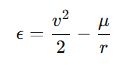
where:
-

For bound orbits:

For 3I/ATLAS:

This confirms extrasolar origin beyond any reasonable doubt.
2.3 Asymptotic Velocity
The hyperbolic excess velocity:
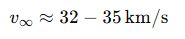
Such a velocity is consistent with:
-
Galactic disk stellar velocity dispersion
-
Ejection from a mature planetary system via giant planet scattering
3. Physical Size, Shape, and Mass Constraints
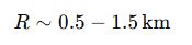
Direct imaging does not resolve the nucleus, but photometric modeling suggests:
-
Effective radius:
-
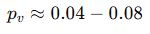
Albedo assumption:
Assuming bulk density:

Estimated mass:
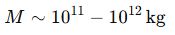
These values are fully compatible with cometary nuclei, though uncertainties remain significant.
4. Spectroscopic Composition and Volatile Chemistry
4.1 Gas Emission Lines
Spectroscopy reveals:
-
Strong CO₂ emission
-
CO detected at higher-than-Solar-System ratios
-
H₂O present but not dominant
The production rates roughly follow:
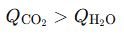
This is unusual compared to most Solar System comets but consistent with formation in colder environments.
4.2 OH Radical Detection
OH emission arises from:

This confirms:
-
Photodissociation processes
-
Active sublimation
-
A volatile-rich body, not an inert asteroid
5. Thermophysical Modeling
Surface temperature approximation:
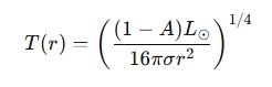
At perihelion (r∼1.3 AU) :

This temperature range allows:
-
CO₂ and CO sublimation
-
Dust entrainment
-
Formation of an extended coma
No anomalous thermal excess has been detected.
6. Plasma Interaction and X-Ray Emission
X-ray emission detected around 3I/ATLAS is consistent with solar wind charge exchange (SWCX):

Observed X-ray halo:
-
Spatial extent: ~400,000 km
-
Luminosity: consistent with cometary models
-
No coherent or pulsed emission
This strongly supports a natural plasma interaction, not an engineered signal.
7. Comparison with Previous Interstellar Objects
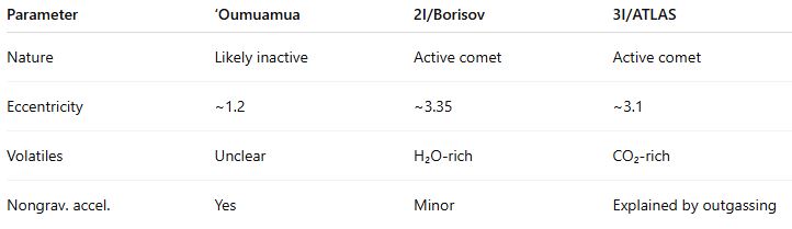
3I/ATLAS appears to be the most chemically exotic ISO observed so far.
8. Theoretical Space for Non-Standard Interpretations
8.1 Why Speculation Exists
Speculation arises because:
-
ISOs are statistically rare
-
Limited observation time
-
Unknown formation environments
-
Prior precedent (ʻOumuamua anomalies)
8.2 Constraints on Artificial Origin
Any artificial hypothesis must explain:
-
Lack of structured radio emissions
-
No coherent acceleration signatures
-
No metallic spectral lines
-
Coma chemistry matching volatile sublimation
To date:
Natural models≫Artificial models\text{Natural models} \gg \text{Artificial models}
by orders of magnitude in explanatory power.
9. Scientific Significance
3I/ATLAS provides:
-
Direct sampling of extrasolar planetesimal chemistry
-
Constraints on planetary system ejection efficiency
-
Data for galactic population models of ISOs
-
A benchmark for future interstellar intercept missions
10. Conclusion
From a rigorous astrophysical standpoint, 3I/ATLAS is best explained as a volatile-rich interstellar comet, ejected billions of years ago from an unknown planetary system.
Yet its rarity, alien chemistry, and fleeting passage remind us that our Solar System is not isolated, and that the line between the known and the unknown remains fertile ground for both science and imagination.
The object does not require exotic explanations — but it invites them, and science advances precisely by knowing where imagination must stop and evidence must begin.
Artificial Intelligence on Aircrafts
Exploring the Role of Artificial Intelligence in Modern Aircraft Systems
Artificial Intelligence (AI) has been making waves in various sectors, and the aviation industry is no exception. The integration of AI in modern aircraft systems is revolutionizing the way we fly, enhancing safety, efficiency, and overall passenger experience. This article explores the role of AI in modern aircraft systems, shedding light on how this technology is shaping the future of aviation.
AI’s primary role in modern aircraft systems is to enhance safety. It achieves this by improving the accuracy of flight operations and reducing human error, which is a significant cause of aviation accidents. AI systems can analyze vast amounts of data in real-time, enabling them to predict and prevent potential issues before they occur. For instance, AI can monitor engine performance and alert the crew to any anomalies that could lead to malfunctions. This predictive maintenance capability not only enhances safety but also reduces downtime and maintenance costs.
Moreover, AI is instrumental in improving flight efficiency. It can optimize flight paths based on real-time weather data and air traffic, reducing fuel consumption and flight times. AI can also automate routine tasks, freeing up the crew to focus on more critical aspects of the flight. For example, AI can handle tasks such as adjusting the aircraft’s altitude or speed, allowing the pilot to concentrate on navigating through complex airspaces.
AI’s role extends beyond the cockpit, enhancing the passenger experience as well. AI-powered chatbots can provide passengers with real-time flight updates, answer queries, and even assist with check-in procedures. Onboard, AI can personalize the in-flight entertainment system based on passenger preferences, making the journey more enjoyable. Furthermore, AI can analyze passenger feedback to identify areas of improvement, helping airlines to continually enhance their services.
The integration of AI in modern aircraft systems also has significant implications for pilot training. AI-powered flight simulators can provide a realistic training environment, allowing pilots to gain experience in handling various flight scenarios. These simulators can adapt to the trainee’s skill level, providing personalized training that enhances learning outcomes. Additionally, AI can analyze the trainee’s performance, identifying areas of weakness and suggesting targeted training to address these areas.
However, the use of AI in aviation is not without challenges. Concerns about data privacy and security are paramount, given the sensitive nature of the data involved. There is also the question of accountability in the event of an AI system failure. As such, robust regulatory frameworks are needed to address these issues and ensure the safe and ethical use of AI in aviation.
In conclusion, AI is playing a pivotal role in modern aircraft systems, enhancing safety, efficiency, and passenger experience. It is also transforming pilot training, providing a more effective and personalized learning environment. However, the integration of AI in aviation also presents challenges that need to be addressed. As the aviation industry continues to embrace AI, it is crucial to strike a balance between leveraging the benefits of this technology and mitigating its potential risks. With the right approach, AI has the potential to propel the aviation industry into a new era of safety and efficiency.
The Impact of AI on Aircraft Safety and Efficiency

Artificial Intelligence (AI) has been making waves in various industries, and the aviation sector is no exception. The integration of AI in aircraft systems is revolutionizing the way we fly, enhancing safety, and improving efficiency in unprecedented ways.
AI’s impact on aircraft safety is profound. Traditionally, the safety of an aircraft has been heavily reliant on the skills and judgment of the pilot and crew. However, human error has been a significant factor in many aviation accidents. AI technology, with its ability to process vast amounts of data and make complex calculations in real-time, can significantly reduce the risk of human error. For instance, AI can monitor the aircraft’s systems continuously, identifying potential issues before they become critical. It can also assist pilots in making informed decisions during emergencies, thereby enhancing the overall safety of the flight.
Moreover, AI can predict potential mechanical failures by analyzing data from the aircraft’s sensors. This predictive maintenance can prevent unexpected breakdowns and reduce the risk of accidents. AI can also improve the safety of flights by optimizing flight paths to avoid bad weather or turbulence, which not only ensures a smoother ride but also reduces the risk of weather-related incidents.
In addition to safety, AI is also enhancing the efficiency of aircraft operations. One of the ways it does this is through fuel optimization. Fuel consumption is a significant cost factor in aviation, and optimizing it can lead to substantial savings. AI can analyze various factors such as weather, altitude, and flight path to determine the most fuel-efficient route. This not only reduces costs but also contributes to environmental sustainability by reducing carbon emissions.
AI also improves efficiency by streamlining ground operations. For example, AI can optimize the scheduling of flights, crew, and maintenance tasks, reducing delays and improving the overall efficiency of the airline. Furthermore, AI can automate routine tasks, freeing up the crew to focus on more critical aspects of the flight.
AI’s ability to process and analyze vast amounts of data also enables airlines to personalize their services, improving the passenger experience. For instance, AI can analyze passenger data to provide personalized in-flight entertainment or meal choices, enhancing customer satisfaction and loyalty.
However, the integration of AI in aircraft systems is not without challenges. There are concerns about the potential for AI systems to be hacked, leading to security risks. There is also the question of job displacement, as AI could potentially replace human roles in the aviation industry. Moreover, the reliance on AI could lead to a lack of human oversight, which could be problematic in situations where human judgment is crucial.
Despite these challenges, the potential benefits of AI in enhancing aircraft safety and efficiency are undeniable. As AI technology continues to evolve, it is likely to play an increasingly significant role in the aviation industry. The key will be to strike a balance between leveraging the benefits of AI and addressing the associated risks and challenges. This will require ongoing research, robust regulatory frameworks, and a commitment to continuous learning and adaptation. In conclusion, the advent of AI in aviation marks a new era of safer, more efficient, and more personalized air travel.
Future Trends: Artificial Intelligence in Aircraft Design and Navigation
Artificial Intelligence (AI) has been making waves in various industries, and the aviation sector is no exception. The integration of AI in aircraft design and navigation is not only a fascinating development but also a significant stride towards the future of aviation. This article will delve into the future trends of AI in aircraft design and navigation, highlighting how this technology is set to revolutionize the aviation industry.
AI’s role in aircraft design is becoming increasingly prominent. Traditionally, aircraft design has been a labor-intensive and time-consuming process, involving numerous iterations and simulations. However, with the advent of AI, this process is becoming more streamlined and efficient. AI algorithms can analyze vast amounts of data from previous designs and simulations, learning from them to create optimized designs. This not only reduces the time taken to design an aircraft but also results in more efficient and safer aircraft. Furthermore, AI can also predict potential design flaws that might not be apparent to human designers, thereby further enhancing the safety of the aircraft.
In addition to aircraft design, AI is also making significant strides in aircraft navigation. AI-powered autopilot systems are becoming increasingly sophisticated, capable of handling a wide range of flight scenarios. These systems can analyze real-time data from various sensors and instruments on the aircraft, making split-second decisions that can enhance the safety and efficiency of the flight. Moreover, AI can also learn from each flight, continuously improving its decision-making capabilities.
AI is also set to revolutionize air traffic management. Currently, air traffic controllers have to manually coordinate the movements of hundreds of aircraft in the airspace. This is a complex and stressful task, especially during peak times. However, AI can automate this process, analyzing real-time data from all aircraft in the airspace and making optimal decisions to ensure smooth and safe air traffic flow. This not only reduces the workload on air traffic controllers but also enhances the overall efficiency of air traffic management.
Furthermore, AI can also play a crucial role in predictive maintenance of aircraft. By analyzing data from various sensors and systems on the aircraft, AI can predict potential failures before they occur. This allows for proactive maintenance, reducing downtime and enhancing the overall reliability of the aircraft.
However, the integration of AI in aircraft design and navigation also presents certain challenges. One of the main concerns is the reliability of AI systems. While AI algorithms are capable of learning and improving over time, they are not infallible. There is always the risk of AI systems making incorrect decisions, which can have serious consequences in the aviation industry. Therefore, it is crucial to have robust checks and balances in place to ensure the reliability of AI systems.
In conclusion, the future of AI in aircraft design and navigation is promising, with the potential to revolutionize the aviation industry. However, it is also crucial to address the challenges associated with AI integration to ensure the safety and efficiency of aircraft operations. As we continue to explore the potential of AI in aviation, it is clear that this technology will play a pivotal role in shaping the future of the industry.
Solutions to make aviation industry turbulence-free
Austrian firm Turbulence Solutions aims to eliminate air turbulence by reducing turbulence loads felt by passengers by over 80% through counteracting control surface deflections. The company’s goal is to mature the technology and establish partnerships to make the entire aviation industry turbulence-free, including airliners. Turbulence Cancelling creates counter turbulence to steady an aircraft’s motion as it flies by installing sensors and small flaps to the aircraft’s wings. The flaps quickly generate vertical lift to counteract turbulence when needed, deflecting turbulent airflow for a smoother ride.
The company’s journey began with the patented invention ‘Improved Direct Lift Control,’ which enables very fast lift generation. Turbulence Solutions has installed the system on a light aircraft, with promising results so far. The company plans to expand across the entire aviation industry and work on large commercial airliners.
Turbulence Solutions has a clear timeline for its expansion across the aviation industry, with the system being widely available for light aircraft next year, eVTOL air taxis by around 2026, private jets in 2028, and commercial airliners by around 2030. The company is addressing a growing problem, with intense turbulence increasing by 55% over the North Atlantic over the past four decades and becoming more common due to climate change.
How to calculate Weight and Balance -Calculation tool
Weight and Balance Calculation
This article deals with weight and balance calculation for aircraft, a crucial pre-flight skill for pilots. it’s a basic and easy calculation that becomes second nature. As pilots move into larger aircraft, the task becomes more challenging. Practice makes it non-negotiable. Weight and balance calculations don’t require complex math or hours of hard work, and can be done quickly with a step-by-step guide. New technology like ForeFlight makes these calculations easier.
[sg_popup id=165090]
Why Calculate Weight and Balance?
Weight and balance are crucial for aircraft performance and safety, as they limit the aircraft’s capabilities. Regulations do not explicitly require calculations of weight and balance before every flight, but they are implied. The maximum takeoff weight is the most important number, and operating beyond this can result in negative flight characteristics such as higher takeoff speeds, longer landing rolls, reduced performance, higher stall speeds, exceeded limits on landing gear and brakes, and more load on the aircraft’s structure.
To ensure balance, find the loaded airplane Center of Gravity (CG) and compare it to the manufacturer’s charts or tables. The CG should not be too far forward or too far back, as either can make the airplane dangerous and unstable. A CG located forward of the forward limit can cause a nose-down tendency, increasing stall speed and making cruise flight slower. A CG located too far aft can cause a nose-up tendency, increasing cruise speed but making the aircraft less stable. If the airplane begins pitching up and slowing, it may be impossible for the pilot to lower the nose, reduce the angle of attack, and recover. A rearward out-of-limits CG is associated with unrecoverable stalls and spins.
Weight and Balance Terms
Standard empty weight — The weight of the airframe, engines, and permanently installed fixtures and fluids (including unusable fuel and full engine oil)
Basic empty weight — Standard empty weight plus any accessories your airplane might have added
Licensed empty weight — An older term than “standard empty weight,” which does not include engine oil
Maximum ramp weight — Total loaded aircraft weight only published for some airplanes. This will be a few pounds heavier than maximum takeoff weight because it assumes you will burn some for taxi and run-up.
Maximum takeoff weight — Maximum weight you can take off with.
Maximum landing weight — Maximum weight you can land with. This is not always published, or it may be published as equal to takeoff weight. Larger aircraft have landing weights much less than takeoff weights since they are designed to burn hundreds (or thousands) of pounds of fuel during flight.
Maximum zero fuel weight — The loaded aircraft weight with everything except fuel. Only published for some aircraft. This is a loading figure to reduce stress on the wings.
Payload — A common term for the maximum weight an airplane can carry of things that can pay the bill—passengers or cargo.
Useful load — A common term for what an airplane can carry that the pilot loads aboard—pilot, passengers, cargo, and fuel. It is found by taking the maximum takeoff weight and subtracting out the aircraft’s basic empty weight.
Datum — A reference point chosen by the manufacturer from which all arms are measured. Where it doesn’t matter, but it is usually located at the tip of the propeller spinner or the engine firewall.
Arm — The distance measured fore or aft of the datum. Every location a pilot can load an object will have an arm distance listed in the AFM (Aircraft Flight Manual). If an arm is located forward of the datum, it will be a negative number.
Station — A location in the airplane where you can load something. Examples of stations include front seats, rear seats, main baggage area, nose baggage area, fuel tanks, etc.
CG — The center of gravity measured in inches aft of the datum. The airplane will have a minimum and maximum CG location for every available weight.
Moment — A measurement of the force that an item places on the airplane. A 100-pound object will produce more force the farther away from the datum that it is located. In other words, a 100-pound bag will affect your CG location more the farther back in the airplane it is located. Moments are measured in inch-pounds.
Moment index — Moments are usually long numbers, so many AFMs index them to simplify the math. This simply means they divide them by either 100 or 1,000. So 224,537.0 in-lbs becomes 2,245.37 or 224.537.
Finding the Weight and Balance with the Calculation Method
Make Your Table
To calculate weight and balance, create a blank table for each item, filling in columns “weights,” “arm,” and “moments.” Write the weight and balance formula at the top for reminder. Schools and FBOs (Fixed-base operator) often provide a planning sheet.
Weight x Arm = Moments
The usual line items will be as follows. The list will depend on the available stations for loading in your aircraft. The first line will always be the empty weight of the airplane.

Step 1: Find the Aircraft’s Empty Weight
To complete the table for an airplane, ensure you know the airplane’s AFM, where is written the last time a mechanic physically weighed the aircraft. Use this record to obtain the empty weight and total moments, and add them to the first row of your table.
Step 2: Weight Your Gear and Passengers
In a small airplane, use exact numbers for weight calculations. Ask passengers about their weight and use a scale if they don’t know. Include heavy jackets and boots for winter. Multiply the gallons of fuel by 6 to calculate avgas weight. Include all non-bolted items, such as flight bags, spare parts, oil, and baggage items. Remember to include everything not bolted down, such as flight bags, spare parts, and oil.
Step 3: Do the multiplication for each row to calculate the moment.
Step 4: Find Total Weight
Se hai superato il peso massimo al decollo, potresti dover lasciare alcuni oggetti (o persone!) dietro. Oppure potresti prendere in considerazione l’idea di partire con meno carburante se è sicuro farlo
Step 5 – Find Total Moment and CG
Your AFM will provide a way to find whether or not the airplane is in balance. It will provide the answer using the total moments, total arm (CG), total weight. The CG (Center of Gravity) is calculated as total moment divided by the total weight. Usually a graph method is used, by means you can verify if Total Weight and CG are within the “safety area” (delimited by closed lines, see figure below).

As well as the CG of airplane with Zero Fuel has to be calculate. The Zero Fuel indicated by blue dot in figure above, can be considered conservatively as landing phase of aircraft.
The “safety area” delimited by closed lines reported above, is provided by the AFM. The “safety area” is determined by a table (in the tool below is named as “CG Envelope Table”).
Below the tool to calculated the Weight and Balance (click on “N172XX Cessna 172M Example” or “ADD NEW AIRCRAFT PROFILE” if you want to change also the “CG Envelope Table”/”Safety area”).
[netleader_aviator]
AI in the Aerospace Industry
AI in the Aerospace Industry
AI is expected to revolutionize the aerospace sector over the next 15 years by reducing costs, reducing design process length, and improving production processes. However, there is limited adoption due to lack of access to high-quality data, reliance on simple models, and lack of experienced personnel. AI can be a game-changing breakthrough in productivity, efficiency, speed, and development for aerospace firms. Applications include analytics, software configuration, customer service, finance, advertising, retail, and health. AI can expedite manufacturing, address safety concerns, and process large volumes of data faster than humans. AI in aircraft can also aid in fuel savings, improvement identification, and air traffic management. Companies like Raytheon, General Dynamics, and Northrop Grumman have announced AI-based development initiatives and product launches.
Below mentioned are some of the applications that are making the aerospace industry disruptive using AI technology.
1. Product Designing
The aviation industry is increasingly utilizing generative structures and AI algorithms to create economical and robust airplane parts. This iterative process, which involves input from designers and constraints like materials and budget, can be combined with AI to quickly explore multiple design options, leading to the creation of lightweight, cost-effective products like propellers and wings. AI can help optimize architecture and manufacturing processes in the aerospace industry.
2. Better Fuel Efficiency
Fuel quality is crucial for aerospace industries, and reducing fuel usage can significantly impact a company’s bottom line and sustainability. A typical commercial flight uses around 4 litres per second, 240 litres per minute, and 14 400 litres per hour of fuel. AI technology can reduce fuel usage by 5 to 7%, as demonstrated by Safety Line’s machine learning program. This program can improve pilots’ climbing trajectories, which consume the most gasoline, saving money on fuel consumption.
3. Supply Chain Management
AI integration in aeronautics distribution streamlines business by improving supply chain competence, making maintenance and repairs easier, saving money, and reducing downtime. Automated data collection can enhance supply chain management competency quickly, enhancing efficiency and efficiency.
4. Training & Practices
AI can be used in flight training by combining simulations with interactive virtual frameworks. It can also gather and evaluate educational data to create tailored training patterns. AI can also assist pilots during flying by optimizing flight paths based on fuel levels, framework state, and weather conditions. Additionally, planes equipped with powerful cameras can enhance pilots’ sight field and performance.
5. Improve Customer Experience
In commercial aviation, AI can enhance customer satisfaction and service quality by utilizing chatbots, AI-powered automated systems that answer customer questions in a human-like manner. These automated systems can save time and effort by automating customer care. This can be done in a number of different ways:
- Chatbots using AI provide quick and polite assistance
- Automatic Assistance is available 24×7
- Customer contacts more efficient
6. Air Traffic Management
Air traffic control is crucial for airports and airlines, but it can become complex due to billions of passengers. AI can help manage air traffic by using weather and flight data to make informed decisions. AI-powered smart assistants can offer different routes, making air transportation safer and faster. AI and smart cameras can also help identify planes leaving the runway, alerting flight attendants and clearing the touchdown runway. This technology can be particularly useful in low-visibility situations like fog.
7. Identification of Threats
AI can be used to identify and categorize hazards and dangers using computer vision systems, advanced analytics, and geospatial signal processing. Images and videos from aerial vehicles and satellites can be trained to classify risks as regular or suspicious. AI-based applications benefit commercial, civic, and commercial applications. Incorporating AI into the aerospace industry can help pilots make informed decisions based on spatial and situational information.
8. Passenger Identification
AI can enhance security in commercial airlines by utilizing facial recognition in airport smart cameras to identify questionable individuals, potentially using images of criminally charged individuals to train AI systems for criminal behavior detection.
Conclusion
AI and machine learning are rapidly expanding their applications in aviation, from automatic detect-and-avoid technologies to computerized air traffic management and combat tactics. These technologies provide enhanced customer experiences through mechanization and self-service apps, enabling aerospace businesses to make better discounts and competitive positioning. Machine learning improves cost and safety, enhances air safety, and reduces employee productivity. It also provides valuable knowledge that traditional methods may not offer, advancing the aircraft sector and enhancing overall efficiency.
Indian rover begins exploring Moon’s south pole – How it works
Indian rover begins exploring Moon’s south pole – How it works
India has successfully launched its Chandrayaan-3 rover, marking the first time the country has landed a craft near the lunar south pole. The six-wheeled, solar-powered rover will amble around the region, transmitting images and scientific data over its two-week lifespan.
The Chandrayaan-3 mission, which aims to explore the Moon’s surface, follows a Russian lander crash in the same region and the previous Indian lunar mission’s failure in final descent four years ago. India is now matched by established spacefaring nations, with Chandrayaan-3 attracting public attention since its launch six weeks ago.
Indian Prime Minister Narendra Modi praised the successful lunar landing, a feat only achieved by the US, Russia, and China. SpaceX’s Elon Musk praised the landing as “super cool”. The Indian mission took longer than the Apollo missions in the 1960s and 1970s, as Chandraaan-3 was launched on a less-powerful rocket and had to orbit Earth multiple times to gain speed.
What challenges does the mission face?
India’s Chandrayaan-3 mission, which aims to land on the lunar south pole, has faced challenges due to rough terrain. ISRO scientists have made adjustments to improve the landing chances, including a broadening of the landing zone and a lander with more fuel and sturdier legs. Russia’s Luna-25 spacecraft also failed, and ispace, a private Japanese space startup, also failed an attempt in April.
How it Works
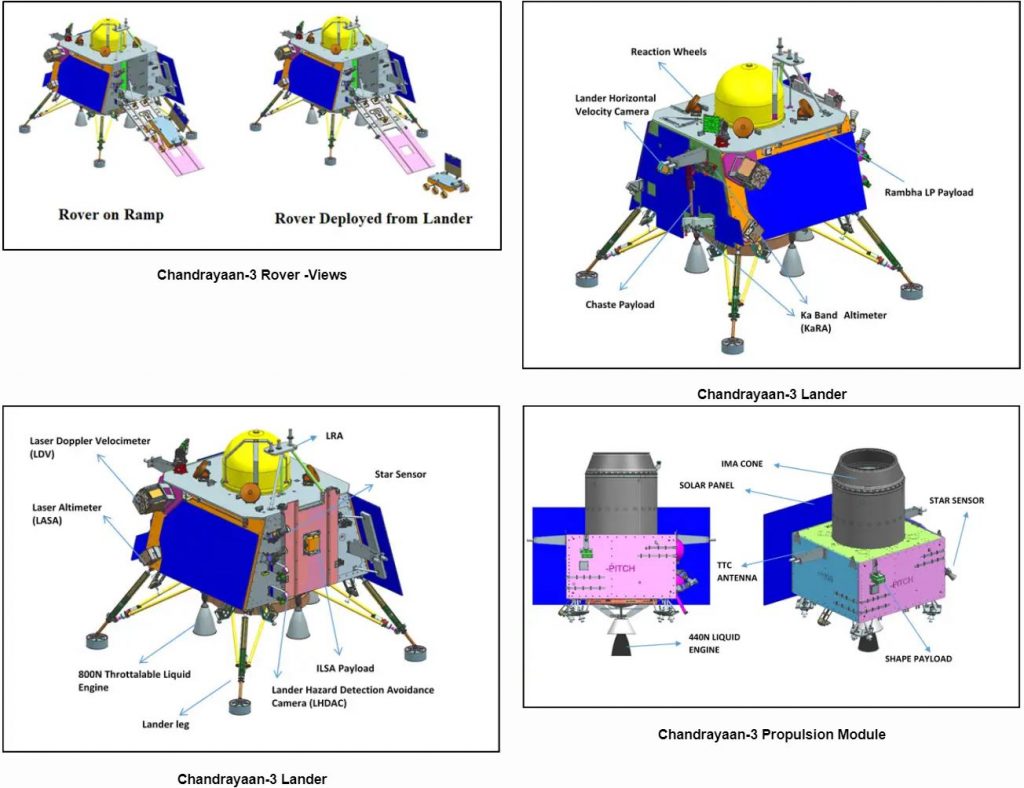
Chandrayaan-3 is a follow-on mission to Chandrayaan-2 to demonstrate end-to-end capability in safe landing and roving on the lunar surface. It consists of Lander and Rover configuration. It will be launched by LVM3 from SDSC SHAR, Sriharikota. The propulsion module will carry the lander and rover configuration till 100 km lunar orbit. The propulsion module has Spectro-polarimetry of Habitable Planet Earth (SHAPE) payload to study the spectral and Polari metric measurements of Earth from the lunar orbit.
Lander payloads: Chandra’s Surface Thermophysical Experiment (ChaSTE) to measure the thermal conductivity and temperature; Instrument for Lunar Seismic Activity (ILSA) for measuring the seismicity around the landing site; Langmuir Probe (LP) to estimate the plasma density and its variations. A passive Laser Retroreflector Array from NASA is accommodated for lunar laser ranging studies.
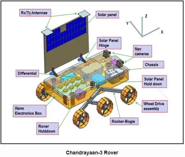
Rover payloads: Alpha Particle X-ray Spectrometer (APXS) and Laser Induced Breakdown Spectroscope (LIBS) for deriving the elemental composition in the vicinity of landing site.
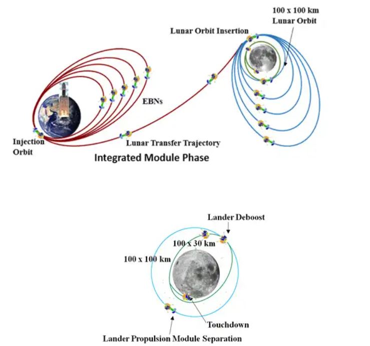
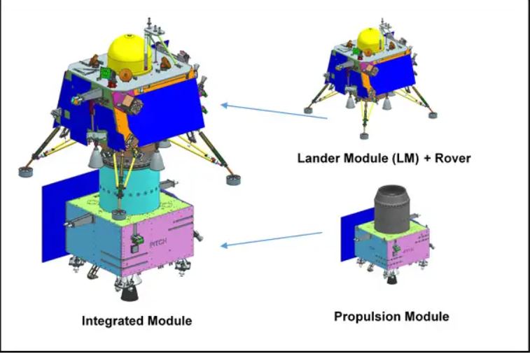
Chandrayaan-3 consists of an indigenous Lander module (LM), Propulsion module (PM) and a Rover with an objective of developing and demonstrating new technologies required for Inter planetary missions. The Lander will have the capability to soft land at a specified lunar site and deploy the Rover which will carry out in-situ chemical analysis of the lunar surface during the course of its mobility. The Lander and the Rover have scientific payloads to carry out experiments on the lunar surface. The main function of PM is to carry the LM from launch vehicle injection till final lunar 100 km circular polar orbit and separate the LM from PM. Apart from this, the Propulsion Module also has one scientific payload as a value addition which will be operated post separation of Lander Module. The launcher identified for Chandrayaan-3 is LVM3 M4 which will place the integrated module in an Elliptic Parking Orbit (EPO) of size ~170 x 36500 km.
To achieve the mission objectives, several advanced technologies are present in Lander such as,
- Altimeters: Laser & RF based Altimeters
- Velocimeters: Laser Doppler Velocimeter & Lander Horizontal Velocity Camera
- Inertial Measurement: Laser Gyro based Inertial referencing and Accelerometer package
- Propulsion System: 800N Throttleable Liquid Engines, 58N attitude thrusters & Throttleable Engine Control Electronics
- Navigation, Guidance & Control (NGC): Powered Descent Trajectory design and associate software elements
- Hazard Detection and Avoidance: Lander Hazard Detection & Avoidance Camera and Processing Algorithm
- Landing Leg Mechanism.
Future Goals
India’s low-budget space program, Chandrayaan-3, has grown significantly since its 2008 lunar landing. The mission cost $74.6 million, significantly lower than many other countries. India’s frugal space engineering is attributed to copying and adapting existing technology and employing skilled engineers.
In 2014, India became the first Asian nation to orbit Mars and plans to send a probe towards the sun in September. ISRO plans a three-day crewed mission into Earth’s orbit by next year, a joint mission with Japan to send another probe to the Moon by 2025, and an orbital mission to Venus within two years.