
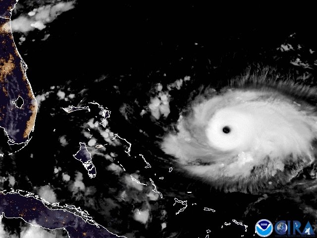
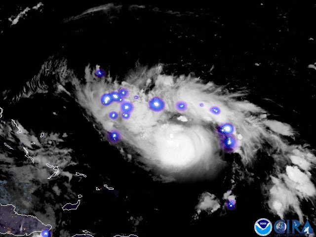
NOAA’s #GOESEast spotted lightning in the eye of #HurricaneDorian this morning. The now catastrophic Cat. 5 storm is expected to bring life-threatening storm surge and very heavy rainfall to the Abaco Islands and Grand Bahama through Monday. More: http://go.usa.gov/xVKrj
The Most Launched Rocket – History Of The R-7
First launched in 1957, the R-7 was the biggest leap in the world’s rocketry since the German A-4. Ironically, developed to be the first Soviet Intercontinental Ballistic Missile, ICBM, the R-7 had become obsolete as a weapon even before it started flying. Yet, as a launch-vehicle, it has continued serving the Russian space program for more than half a century after it was originally conceived. In the 21st century, the R-7-derived space boosters remain only vehicles delivering Russian manned spacecraft into orbit. The assemby of the International Space Stationalso depended on the R-7-based rocket, launching supply ships and lifeboats for the outpost’s crews.
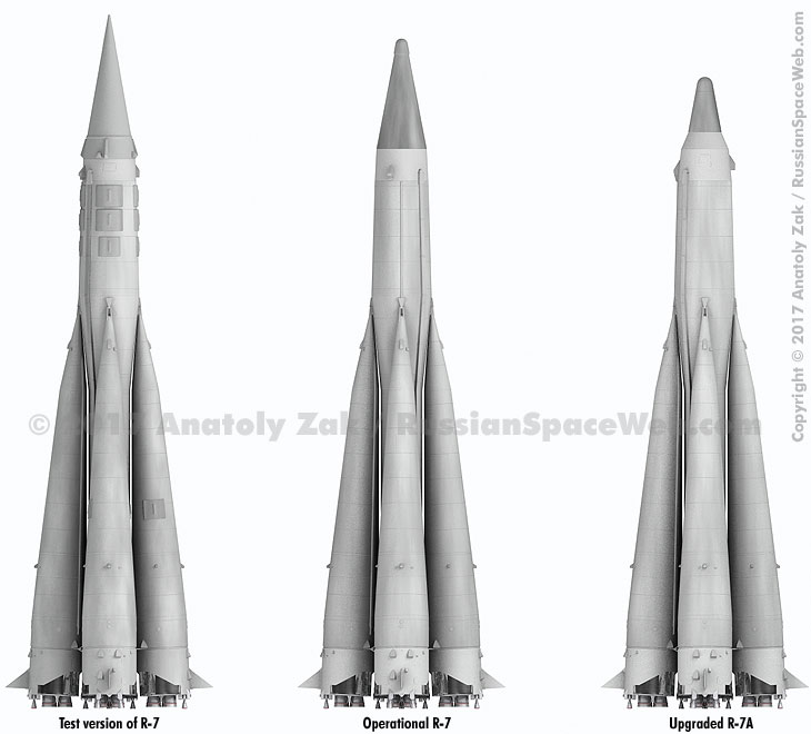
The R-7 family of intercontinental ballistic missiles with industrial designation 8K71.
Known technical specifications of the R-7 ICBM:
|
Number of stages
|
2
|
|
Length of the vehicle
|
|
|
Diameter
|
10.3-11.2 meters at the base of four strap-on boosters
|
|
Weight (fueled)
|
280 tons (empty weight: 27 tons)
|
|
Fuel
|
Kerosene T-1
|
| Oxidizer | Liquid Oxygen |
| Weight of propellant | 253 tons |
| First launch | 1957 |
| Launch sites | Tyuratam (two pads), Plesetsk (four pads) |
|
Flight range: |
8,500-8,800 (8,000) km
|
|
Warhead type (single):
|
KB-11-developed – 5,300-5,500-kg, 7.27-meter, 3-5 megaton, thermonuclear
|
|
Accuracy
|
2.5-5.0 kilometers (max. deviation 10 kilometers)
|
|
Officially in armaments
|
R-7 (8K71) since January 20, 1960 until mid-1960s
|
| Stage 1 | Four strap-on booster (Blocks B, V, G, D) |
| Stage 1 weight | 170 tons |
| Stage 1 length | 19.2 meters |
| Stage 1 diameter | 2.68 meters |
| Stage 1 burn time | 104-130 seconds from launch |
| 1st stage propulsion |
|
| Stage 2 | Core (Block A) |
| Stage 2 weight (fueled) | 93.36 tons |
| Stage 2 dry weight | 6.465 tons |
| Stage 2 length | 28 meters |
| Stage 2 diameter | 2.95 meters |
| Stage 2 burn time | 285-320 seconds |
| 2nd stage propulsion |
|
| Launch system | ground-based: Tyulpan (8U215) |
| Storage time (fueled) | 30 days |
| Readiness time | 2 hours |
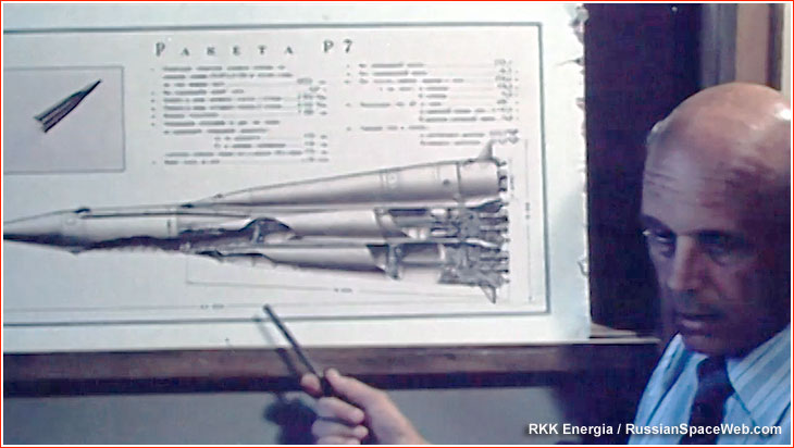
Sergey Kryukov, a key engineer behind the R-7.
The R-7 development team:
| Element | Developer | Chief-designer | Location |
| Overall design |
OKB-1
|
S. P. Korolev
|
Podlipki (Korolev)
|
| Production (initial) |
Zavod No. 88
|
–
|
Podlipki (Korolev)
|
| Production (serial) |
Zavod No. 1 Progress
|
D.I. Kozlov
|
Kuibyshev (Samara)
|
| Propulsion units (both stages) |
OKB-456
|
V. Glushko
|
Moscow
|
| Control system |
NII-885
|
N. Pilugin
|
Moscow
|
| Launch complex (surface) |
KB-59 Kompressor
|
V.P. Barmin
|
Moscow
|
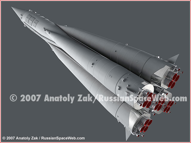
General configuration of the R-7 ICBM.
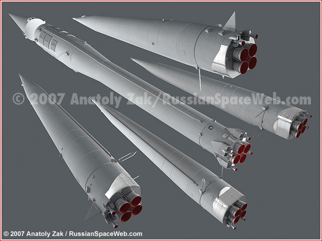
Main components of the R-7 rocket.
Early milestones in the R-7 program (Phase I of flight testing and orbital launch attempts):
First test mission
The first R-7 missile (Number 5L) arrived at Tyuratam on March 3, 1957. After pre-launch processing at Site 2, it was rolled out to the launch pad at Site 1 in the yearly hours of May 5, 1957. Key officials in charge of the program, walked by the transporter/erector all the way to the launch pad, starting a long tradition of future Soviet space launches.
1957 May 15, 19:01 Moscow Time: The first R-7 lifted off from Baikonur. It was programmed to fly a standard test distance of 6,314.5 kilometers, however failed and crashed 3,197 kilometers downrange, deviating 12.6 kilometers from the nominal flight path. Western sources suggested that the vehicle failed after around 20 seconds, however post-Cold War Russian memoirs revealed that although the fire in the tail section of the rocket developed shortly after the launch, controlled flight went on until T+98 seconds and the emergency shutdown of the engines took place around 100 seconds after liftoff.
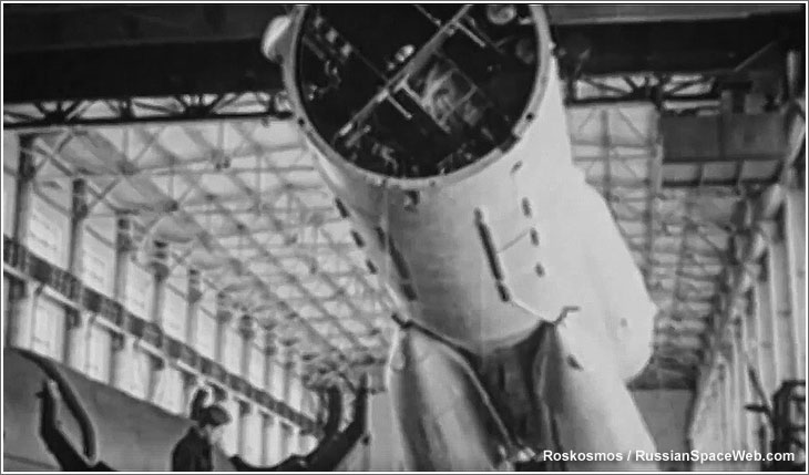
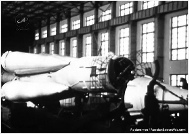
An R-7 missile being integrated with the original version of its warhead.
Problems with the second rocket
During June 10-11, 1957, there were three attempts to launch the R-7 rocket (Number M1-6). However the missile remained grounded due to technical problems. It was ultimately removed from the pad and eventually used as a training vehicle.
Third rocket, second launch

1957 July 12, 15:53: The R-7 rocket (Number M1-7) lifted off from Baikonur. The vehicle disintegrated at 32.9 seconds in flight. Its debris crashed about seven kilometers downrange (four kilometers, according to other sources).
Flight 3: almost a success
1957 Aug. 21, 15:25: The R-7 rocket (Number M1-9) launch from Baikonur. Flight went normally, but the warhead disintegrated at the altitude of around 10 kilometers over Kamchatka Peninsula. Despite a mishap at the end of the mission, on August 27, 1957, TASS officially announced “…the creation of a long-range multistage ballistic missile in the Soviet Union.” The announcement went largely unnoticed in the West.
Flight 4
1957 Sept. 7, 14:39: The R-7 (Number M1-10) was launched from Baikonur. Flight went normally, but the warhead section apparently collided with the core stage during the separation and disintegrated again during the reentry. According to recollections of Aleksandr Aleksandrov, the vehicle carried the head section simulating the planned satellite payload. (815)
The First Artificial Satellite of the Earth, Sputnik-1
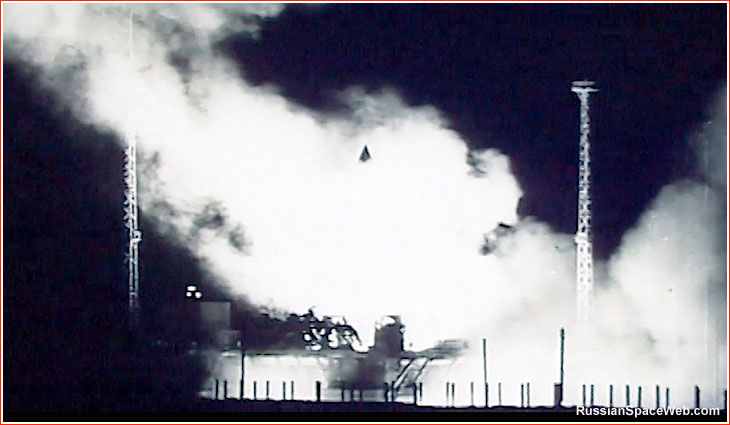
1957 Oct. 4, 22:28:34 Moscow time (00:28:34 local time on October 5): The R-7 rocket (Number 8K71PS) launched world’s first artificial satellite PS-1 or Sputnik-1 from Baikonur.
Second Artificial Satellite of the Earth, Sputnik-2 with dog Laika onboard
1957 Nov. 3, 05:30:42 Moscow time: The R-7 rocket launched Sputnik-2 carrying dog Laika onboard from Baikonur. Laika died three days after the launch from overheating of her cabin. The spacecraft had no reentry system onboard.
Test flights of the R-7 rocket continue
1957 Dec. 22: The R-7 rocket (8K71 Number 11) arrived at Baikonur. Its first launch attempt took place on Dec. 31, 1957, but it was scrubbed.
1958 Jan. 30, 00:15: Test launch of the R-7 rocket (8K71 Number 11) with the M1-12 warhead.
1958 March 12, 22:30: The attempt to launch the R-7 rocket (8K71 Number 6), which was removed from the pad in June 1957, failed again shortly after ignition of the first stage engines. The launch was aborted safely and the rocket was shipped back to the manufacturer.
1958 March 29, 17:40: Launch of the 8K71 (No. 10) with the M1-6A warhead, which became the first to reach its impact area without disintegrating in the air. It was the first launch taking advantage of the Kvarts computer, calculating the trajectory of the flight based on radar data. (644)
1958 April 4, 18:30: Launch of the 8K71 (No. 12) with the B1-11 warhead. Slight overflight of the target with some flight control problems.
Third Artificial Satellite of the Earth, Sputnik-3
1958 April 27, 12:01: Launch of the 8A91 B1-2 launch vehicle, carrying the Object D satellite. The rocket disintegrated 96.5 seconds after the launch.
1958 May 15, 10:00:35.5: Launch of the 8A91 No. B1-1 rocket, carrying a second version of the Object D satellite. After successful orbital insertion, it was announced by the USSR as the Third Artificial Satellite, or Sputnik-3. (51)
Test launches of the R-7 ICBM and its upgraded version known as R-7A continued in Baikonur during 1958 and 1959. According to one source, the test flights during the second half of 1958 and the entire 1959 apparently carried payloads code-named Sliva (plum) and Grusha (pear).
First attempts to hit the Moon
1958 Sept. 23: An R-7-based 8K72 No. B1-3 launch vehicle fails 93 seconds after liftoff during an attempt to send the E1 No. 1 probe to impact the Moon.
1958 Oct. 12: An R-7-based 8K72 No. B1-4 launch vehicle fails 104 seconds after liftoff during an attempt to send the E1 No. 1 probe to impact the Moon.
1958 Dec. 4: An R-7-based 8K72 No. B1-5 launch vehicle fails 245.4 seconds in flight during an attempt to send the E1 No. 1 probe to impact the Moon.
R-7 declared operational
1960 Jan. 20: The R-7 ICBM enters armaments of the Soviet Strategic Missile Forces, RVSN.
Posted in Propulsion, Space Flight
Tagged engine, R-7, rocket, russian, Soyuz, Space, Video
Leave a comment
How Does Quantum Computer Works?
Quantum Computing
Quantum computing often grabs the headlines. The word “quantum” itself is intriguing enough, and combined with the promise of computational power that surpasses anything we have seen so far it becomes irresistible. But what exactly is quantum computing?
To get to grips with quantum computing, first remember that an ordinary computer works on 0s and 1s. Whatever task you want it to perform, whether it’s calculating a sum or booking a holiday, the underlying process is always the same: an instance of the task is translated into a string of 0s and 1s (the input), which is then processed by an algorithm. A new string of 0s and 1s pops out at the end (the output), which encodes the result. However clever an algorithm might appear, all it ever does is manipulate strings of bits — where each bit is either a 0 or a 1. On the machine level, this either/or dichotomy is represented using electrical circuits which can either be closed, in which case a current flows, or open, in which case there isn’t a current.

The idea of superposition led the physicist Erwin Schrödinger to speculate that a cat in a box could be both dead and alive as long as you don’t look at it. (This cat is definitely alive.)
Quantum computing is based on the fact that, in the microscopic world, things don’t have to be as clear-cut as we’d expect from our macroscopic experience. Tiny particles, such as electrons or photons, can simultaneously take on states that we would normally deem mutually exclusive. They can be in several places at once, for example, and in the case of photons simultaneously exhibit two kinds of polarisation. We never see this superposition of different states in ordinary life because it somehow disappears once a system is observed: when you measure the location of an electron or the polarisation of a photon, all but one of the possible alternatives are eliminated and you will see just one. Nobody knows how that happens, but it does. (You can find out more in Schrödinger’s equation — what is it?)
Superposition frees us of from binary constraints. A quantum computer works with particles that can be in superposition. Rather than representing bits — such particles would represent qubits, which can take on the value 0, or 1, or both simultaneously. “If you do something to [such a quantum system], it’s as though you are doing it simultaneously to 0 and to 1,” explains Richard Jozsa, a pioneer of quantum computing at the University of Cambridge.
Spooky action
You might object that something like superposition could perhaps be achieved using only ordinary classical physics — perhaps by processing two ordinary bits at the same time or something like that — in which case quantum computing wouldn’t be that much more amazing than classical computing. But there is more to quantum physics than just superposition. If you look at a system of more than one qubit, then the individual components aren’t generally independent of each other. Instead, they can be entangled. When you measure one of the qubits in an entangled system of two qubits, for example, then the outcome — whether you see a 0 or a 1 — immediately tells you what you will see when you measure the other qubit. Particles can be entangled even if they are separated in space, a fact that caused Einstein to call entanglement “spooky action at a distance”.
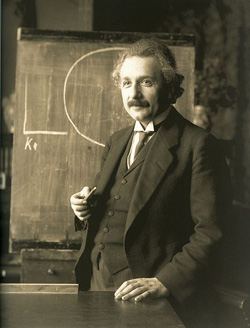
Albert Einstein called entanglement “spooky action at a distance”
Entanglement means that describing a system of several qubits using ordinary classical information, such as bits or numbers, isn’t simply about stringing together the descriptions of the individual qubits. Instead, you need to describe all the correlations between the different qubits. As you increase the number of qubits, the number of those correlations grows exponentially: for n qubits there are 2ncorrelations. This number quickly explodes: to describe a system of 300 qubits you’d already need more numbers than there are atoms in the visible Universe. The idea is that, since you can’t hope to write down the information contained in system of just a few hundred qubits using classical bits, perhaps a computer running on qubits, rather than classical bits, can perform tasks a classical computer can never hope to achieve. This is the real reason why physicists think quantum computing holds such promise.
There’s a hitch however. While a quantum algorithm can take entangled qubits in superposition as input, the output will also usually be a quantum state — and such a state will generally change as soon as you try to observe it. “Nature pulls a trick here,” says Jozsa. “She updates a quantum state, but then she doesn’t allow you to get all the information.” The art of quantum computing is to find ways of gaining as much information as possible from the unobservable.
An example
| Number in decimal | Number in binary |
| 0 | 000 |
| 1 | 001 |
| 2 | 010 |
| 3 | 011 |
| 4 | 100 |
| 5 | 101 |
| 6 | 110 |
| 7 | 111 |
An example of a quantum algorithm is one Jozsa developed together with another pioneer of quantum computing, David Deutsch. The task it performs is slightly curious, but we will think of it as follows. Imagine a line of people waiting at the gates of heaven to see whether they’ll be let in. Guarding those gates is Saint Peter who, in deference to his love for computer science, has labelled all the people with numbers written in binary. There happen to be exactly 23 = 8 people, which means that each person gets their own unique string of three 0s and 1s (see the table above for more about binary numbers). Peter records his decisions by allocating a 1 to a particular bit-string if he is going to let the corresponding person in, and a 0 if he’s not. (Technically this allocation is called a Boolean function, a rule which assigns to each bit-string a 0 or a 1. Boolean functions are a staple of computer science, which is why our example isn’t as far-fetched as it may seem at first.)
You don’t know what Peter is going to decide to do with each individual, but you do know that he’s set in his ways: he’ll either let everybody in (every bit-string gets allocated a 1), or he will let exactly half the people in (half of bit-strings get allocated a 0 and the other half a 1). You task is, not to find out what happens to each individual, but whether Peter is in a generous mood and lets everybody in, or whether he is in a grumpy mood, deciding to let only half of the people in. How many values of Peter’s Boolean function do you need to look up to find out which of the two alternatives it is?
If you work like a classical computer, then in the worst-case scenario you’ll have to look the function up five times. That’s because even if you see a 1 allocated to the first 4 bit-strings you check, you still can’t be sure that all the bit-strings come with a 1: there is still the possibility that it’s only half of them, so you do need that 5th look-up. If you have a quantum computer, however, you can get it to look up the function value for all the eight people simultaneously, so you only need one look-up. “For the cost of running the program once with this funny superposition input, you have somehow computed all the [values at once],” explains Jozsa. This advantage of quantum over classical computation becomes even more apparent when there are more people: for a line consisting of 2n individuals, a classical computer would need to look up the function 2n-1+1 times, a number that grows very quickly with n. A quantum computer would always only need to look once.
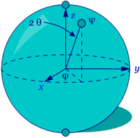
The Bloch sphere is a representation of a qubit, the fundamental building block of quantum computers.
Will quantum computing take us higher?
But then there is nature’s trick: your eight simultaneously-looked-up values will be encoded in a quantum state you can’t actually read, since any measurement of it will disturb it. Luckily, though, you’re not trying to find out what’ll happen to each individual. You only want to know whether Peter is feeling generous our grumpy. “That’s only one yes-no question,” says Jozsa. “It’s a small amount of information about a lot of values.”
Jozsa and Deutsch showed that it’s possible to perform an extra operation on your quantum state, one which teases the simple piece of information you are after into just the right places for you to be able to read it off. It’s a bit like a house of cards that will collapse as soon as you look at it. You might never be able to see it in its full glory, but if it was constructed in just the right way, you may at least be able to ascertain some information on what it looked like from the collapsed heap. And that’s one reason why quantum computers are more powerful than classical ones. To find even simple patterns or structures within systems of many components a classical computer often has no choice but to first evaluate all, or at least many, of the components individually. A quantum computer, on the other hand, can evaluate all of them simultaneously. And although you may not be able to read off all those individual values, you can often extract just enough information to glean a pattern in them.
Jozsa and Deutsch came up with this algorithm in 1992 and it was the first that could be proven to work exponentially faster than any classical algorithm designed to perform the same task. If you’re imagining Jozsa and Deutsch as quantum engineers tinkering away in a lab, however, you couldn’t be further from the truth. Both of them are theorists. They use the mathematical formalism that describes quantum mechanics and theoretical computer science to work out what a combination of the two can achieve. It’s a purely mathematical endeavour — we’re still some way away from actually building fully functional quantum computers that can perform useful tasks. You can find out more in the following articles:
Quantum Algorithms Will Change Cryptography
Superposition and entanglement are impressive physical phenomena, but leveraging them to do computation requires a very different mindset and programming model. You can’t simply throw your C code on a quantum computer and expect it to run, and certainly not to run faster. Fortunately, mathematicians and physicists are way ahead of the computer builders here, having developed clever algorithms that take advantage of quantum computers decades before the machines started to appear.
Some of the first quantum algorithms created, and honestly, some of the few useful ones I’ve found that you can understand without a graduate degree in math, are for secure cryptographic key distribution. These algorithms use the property of entanglement to allow the key creator to send one of each of many pairs of qubits to the recipient. The full explanation is pretty long, but the algorithms rely on the fact that if anyone intercepts and reads one of the entangled bits en route, the companion qubit at the sender will be affected. By passing some statistics back and forth, the sender and receiver can figure out whether the key was transmitted securely, or was hacked on the way.
You may have read that quantum computers one day could break most current cryptography systems. They will be able to do that because there are some very clever algorithms designed to run on quantum computers that can solve a hard math problem, which in turn can be used to factor very large numbers. One of the most famous is Shor’s Factoring Algorithm. The difficulty of factoring large numbers is essential to the security of all public-private key systems — which are the most commonly used today. Current quantum computers don’t have nearly enough qubits to attempt the task, but various experts predict they will within the next 3-8 years. That leads to some potentially dangerous situations, such as if only governments and the super-rich had access to the ultra-secure encryption provided by quantum computers.
Why Building Quantum Computers Is Hard
There are plenty of reasons quantum computers are taking a long time to develop. For starters, you need to find a way to isolate and control a physical object that implements a qubit. That also requires cooling it down to essentially zero (as in .015 degrees Kelvin, in the case of IBM‘s Quantum One). Even at such a low temperature, qubits are only stable (retaining coherence) for a very short time. That greatly limits the flexibility of programmers in how many operations they can perform before needing to read out a result.
Not only do programs need to be constrained, but they need to be run many times, as current qubit implementations have a high error rate. Additionally, entanglement isn’t easy to implement in hardware either. In many designs, only some of the qubits are entangled, so the compiler needs to be smart enough to swap bits around as needed to help simulate a system where all the bits can potentially be entangled.
Getting Started With Quantum Computing
 The good news is that trivial quantum computing programs are actually pretty easy to understand if a bit confusing at first. Plenty of tutorials are available that will help you write your first quantum program, as well as let you run it on a simulator, and possibly even on a real quantum computer.
One of the best places to start is with IBM’s QISKit, a free quantum toolkit from IBM Q Research that includes a visual composer, a simulator, and access to an actual IBM quantum computer after you have your code running on the simulator. Rigetti Quantum Computing has also posted an easy intro application, which relies on their toolkit and can be run on their machines in the cloud.
Unfortunately, the trivial applications are just that: trivial. So simply following along with the code in each example doesn’t really help you master the intricacies of more sophisticated quantum algorithms. That’s a much harder task.
World’s Largest Quantum Computer Doubles Down
The world’s largest maker of quantum computers, Canada’s D-Wave Systems Inc., recently announced the Pegasus generation of its quantum computers, featuring 2.5 times the qubits (more than 5,000) than its predecessor, as well as the elimination of a major stumbling block to commercialization by directly connecting each of those qubits to three times as many nearby qubits as its previous generation, the Chimera.
Analysts are predicting that Pegasus will advance quantum applications down the technology lifetime exponential growthcurve.
Exemplary applications include Denso Corp.’s automated guided vehicles without collision, T-QARD’s factory optimizationcollaboration with Denso, Volkswagen’s intelligent traffic management application, and Los Alamos National Laboratory’s recent mathematical breakthrough showing how to use D-Wave’s quantum annealing architecture to perform quadratic unconstrained binary optimization in place of supercomputer floating point operations.
“D-Wave’s Pegasus opens up new application horizons,” said Bob Sorensen, chief analyst for quantum computing at Hyperion Research. “By adding over twice as many qubits and three times as many interconnections, the quantum annealing operations performed by Pegasus can be adapted to many other applications besides optimization; from machine learning to financial portfolio risk-assessment.”
“Quantum annealing” describes the hardware architecture used by all D-Wave processors. Quantum annealing sidesteps the need for extensive error correction, a problem that plagues the gate-level implementations of Google, IBM, Microsoft, Rigetti, and Xanadu, limiting them to fewer than 70 qubits. Only Fujitsu has also adopted quantum annealing, albeit in a 1024-bit digital chip that only emulates a quantum computer.
According to Sorensen, D-Wave’s Pegasus topology takes it very close to the threshold of commercial growth by virtue of its vastly improved interconnection matrix, in which each qubit is connected to 15 nearby qubits. “Pegasus bridges the gap between quantum computing and real world of applications,” said Sorensen.
The previous generation, Chimera quantum computers, only made direct interconnections between a qubit and five adjacent qubits, forcing programmers to “waste” some of its 2,000 qubits per chip as makeshift interconnections. The new arrangement will allow all 5,000 qubits to be used for equation variables, enabling complex real-world problems to be solved, according to Sorensen.
“For logistics applications, such as optimally routing taxis to riders and their destinations, Pegasus can now handle far more taxis than before,” said Mark Johnson, vice president of processor design and development of quantum products at D-Wave. “Due to its higher connectivity architecture, equation variables can be represented with far fewer qubits. New applications can be taken closer to a positive return-on-investment [ROI], including route scheduling, financial portfolio optimization, and machine learning.”
D-Wave claims that even though its quantum annealing needs no error correction, Pegasus does have improvements in precision that will make a big difference by shortening run times. Quantum annealing works in a manner similar to semiconductor or metallurgical annealing. It’s an iterative process, and each iteration of the annealing process yields a more precise result, so greater precision at each step greatly decreases the overall run time for a given level of precision.
“The increased number of qubits and interconnections is interesting, but the big deal is Pegasus’ higher precision,” said Matthew Brisse, research vice president at Gartner Inc. “There are already over 100 [Chimera] applications on GitHub, but now programmers can accelerate those and their own algorithms by shifting to the new Pegasus topology.”
According to Brisse, it will take five years or more before true quantum supremacy (the potential ability of quantum computing devices to solve problems that classical computers cannot) will be demonstrated on not just scientific, but also on everyday commercial applications.
The software development environment created by D-Wave, called Leap, is already educating programmers on how to best make the transition to quantum, without needing to learn the underlying physics. Programmer efforts are also being spurred by D-Wave’s Ocean code library with standardized Python and C++ application programmer interfaces (APIs) plus Jupyter Notebooks, which allows interactive changes that instantly update results.
Brisse and Sorensen also praised D-Wave for directly responding to its user base when crafting the new Pegasus topology. Most D-Wave users run their quantum algorithms in the cloud, rather than purchasing the company’s hardware. Luckily, D-Wave has unusually patient funding sources, since it is still getting their full support on its 20th birthday.
D-Wave says it was already leading the world in the sophistication of its superconducting process technology, but claims to have extended that lead with a newly enhanced process technology developed with SkyWater Technology, its microchip fabrication foundry. Not only does its current process offer niobium features below 240 nanometers, but also lowers its on-chip noise level, which for a quantum computer translates to longer coherence times—the length of time before data values collapse from a quantum superposition of states into a digital one or zero state. Thus besides enabling more quantum variables to tackle larger problems, according to D-Wave’s Johnson, Pegasus’ lower noise also enables the solution of more complex problems that require longer coherence times to solve.
Finally, Pegasus directly confronts how classical computers and quantum computers work together as companions, rather than as competitors. According to Johnson, hybrid configurations of classical and quantum computers will off-load to Pegasus only the parts of a problem that run better on quantum computers, while retaining a companion classical computer to run the rest of an application’s algorithms. This hybrid architecture has been built into the latest revisions of Leap and its Ocean algorithm library to simplify quantum programming, as well as to demonstrate the best practices needed to perform hybrid classical-quantum computing.
“We really believe that successful customer solutions will be hybrids, so new operating software enhances hybrid configurations with lower latency and new options for scheduling problems,” said Johnson. “In fact, D-Wave is the only company with real-time qubit scheduling, as well as block-of-time scheduling.”
Real-time qubit scheduling allows algorithms to split up classical and quantum operations on a fine-scale, step by step, while block-of-time scheduling permits quantum and/or classical operations to be continuously executed without the overhead of switching modes.
Michael Cusumano at the Massachusetts Institute of Technology (MIT), who is familiar with programming the Chimera generation, says, “D-Wave’s latest machine and programming environment sounds like real progress, and should be exciting for software developers working in the D-Wave ecosystem. Clearly, there are some significant technical advances, and the latest technology may well be closer to a general-purpose quantum computer.”
D-Wave’s Hybrid, for marrying an in-house classical computer to a cloud-based quantum computer, is available on GitHub, as are many of the Pegasus components. The rest of the Pegasus offerings will be rolled out by the company over the next 18 months, according to Johnson.
Posted in Technology & Science
Tagged computing, D-Wave, David, Deutsch, Einstein, equation, Factoring, IBM, QISKit, Quantum, qubit, Schrödinger, Schrödinger's, Spooky, wave
Leave a comment
How does a Soyuz land?
Perhaps the riskiest and scariest part of the Soyuz flight comes at the very end, with the fiery reentry into the atmosphere, followed by a rough touchdown, which, according to many crew members who have experienced it, can only nominally be called soft. The early history of the spacecraft was punctuated by two fatal accidents during the landing of the Soyuz-1 and Soyuz-11 missions, which took lives of four cosmonauts. However, after 1971, the Soyuz has safely brought home all its passengers, despite a few nerve-racking incidents.
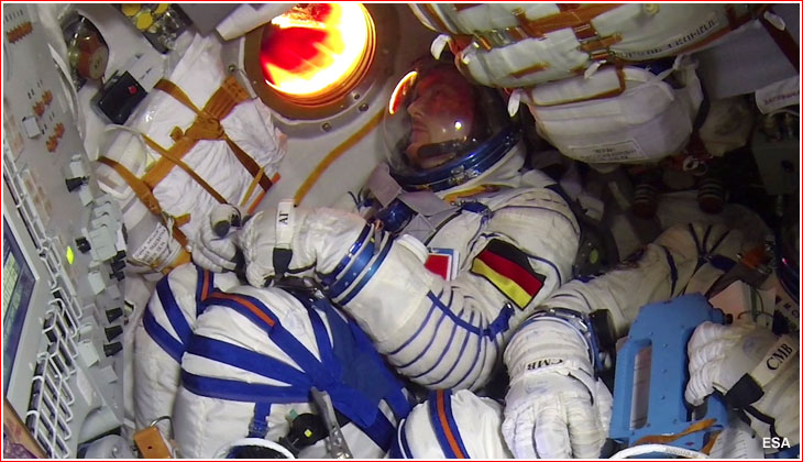
A rare image shows the reentry of the Soyuz TMA-13M mission from the vantage point of the crew inside. A European astronaut Alexander Gerst is enjoying the view.
Undocking from the station
For all Soyuz missions to space stations, the return to Earth begins with undocking. Prior to their departure from the Earth-orbiting outpost, crew members conduct tests of the motion control system in the Soyuz. The crew then boards the vehicle and closes the hatches connecting the transport vehicle and the station, followed by leak checks in the docking port. The hatch between the Descent Module and the Habitation Module is also closed and all crew members, dressed in Sokol launch and entry suits, take seats inside the Descent Module.
On the International Space Station, ISS, the undocking typically takes place during the final (14th or 15th) orbit of a particular day, around 3.5 hours before a scheduled touchdown on Earth. After opening the hooks of the docking mechanism, spring pushers in the docking port give the spacecraft around 0.12 meters per second in relative motion away from the station. The crew monitors the station via an external camera on the Soyuz and makes sure the ship remains in stable flight as it backs away from the outpost.
Around three minutes after undocking, with the two spacecraft around 20 and 30 meters apart, the Soyuz usually performs an eight-second firing of its DPO-B attitude control thrusters delivering between 0.4 and 0.5 meters per second in velocity change to reach a safe distance from the ISS. A similar 15-second maneuver is conducted around a minute later to ensure that the spacecraft will not rendezvous with the station again after one orbit.
Braking maneuver
After two and a half hours in solo flight, when the Soyuz is around half an orbit from its landing site, the spacecraft orients itself tail first in preparation for a braking maneuver, normally conducted over the Southern Pacific and the Atlantic, near the southern tip of South America. Unlike a usual orbit correction, mission control sends a “descent” radio command to the spacecraft prior to the maneuver. In addition, a backup battery is plugged into the main buffer battery, to give the craft maximum “juice” during the remainder of the flight.
Once the ship is flying tail first, the engine cover opens and the main engine fires against the direction of the flight for less than five minutes. The braking maneuver can be conducted in a fully automated mode or it can be initiated manually by the crew, in case of an emergency. If something goes wrong, for example, the spacecraft loses its correct attitude, the crew can abort the maneuver and repeat it during a backup landing opportunity, which is always available. Moreover, attitude control thrusters, DPO-Bs, can finish the job if the main engine quits too early. If necessary, the crew can activate those engines and keep them firing for the necessary duration based on real-time calculations onboard.
If the spacecraft is unable to reach the planned landing site, the crew can still return to Earth with the use of the so-called Mode 14, which is constantly updated when the spacecraft is within the range of ground stations.
Modules’ separation
Based on the “descent” command, the flight control system aboard the Soyuz activates the sequence for the separation of the spacecraft’s modules as soon as it detects that the braking maneuver has been completed.
In preparation for the split of the modules, external cable lines connecting the three main sections of the spacecraft and the six petals of the thermal protection layers on the Descent Module, SA, are shed. The Habitation Module is then depressurized, while the crew members in the Descent Module close the visors on their helmets.
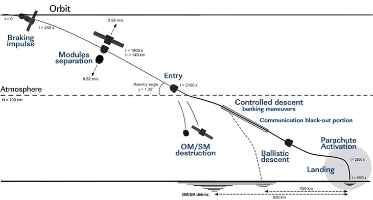
When the spacecraft is in the correct attitude, the Habitation Module, BO, and Instrument Module, PAO, separate from the Descent Module. During a nominal landing, the separation of three modules takes place at an altitude of 140 kilometers over the Arabian Peninsula. The Descent Module with the crew heads for landing, while the two other compartments burn up in the atmosphere.
To ensure that the modules do separate before entering the atmosphere, there is a quadruple backup system. During a nominal flight, the onboard computers of the flight control system, SUDN, issue the separation command automatically. If this doesn’t work, a backup programming timer should activate the so-called Sequence No. 11 to activate separation, also automatically.
If both of these automated systems fail to work, the crew can initiate the process from its console in the capsule.
As a very last resort, signals from thermal sensors on the tail of the vehicle will detect the rising heat from the increasing friction of the Earth’s atmosphere as the spacecraft descends and trigger the separation sequence, though it would take place later than usual.
Right after the separation, a dual VHF PRD radio operating at 121.5 megahertz is activated aboard the Descent Module.
Reentry into the atmosphere
Under normal flight conditions, the Descent Module enters the Earth’s atmosphere under an angle of 1.35 degrees toward the local horizon, at an altitude of around 100 kilometers above the Earth’s surface. By maintaining its correct pitch angle, the capsule can generate some aerodynamic lift, which makes the return trajectory less steep and subjects the crew members to less g-loads than those they would experience in a ballistic descent.
Still, all Soyuz crew members must be prepared for the ballistic return mode (known as BS in Russian), in case of emergency, such as a failure of the flight control or the attitude control system.
In any case, the capsule decelerates sharply as it encounters the dense atmosphere. Around three minutes after the separation of the Descent Module, the air friction causes ablative layers of the capsule to burn, while forming a bubble of plasma around the spacecraft, which makes communications with ground control stations largely impossible for around five minutes 40 seconds, which is long enough for the capsule to descend from an altitude of 90 kilometers to just 35 kilometers.
The flight control system provides the roll of the capsule in order to adjust the landing trajectory. The particular roll angles are calculated by the KSO20M instrument or can be induced by the crew based on indications from the manual control console, RUS. The roll control process is concluded around one minute before the activation of the parachute system.
In case the automated control of the landing trajectory is impossible, but other means for maneuvering the capsule are still functioning, the crew can still try the aerodynamic descent mode or switch to a ballistic mode.
Operation of the parachute system
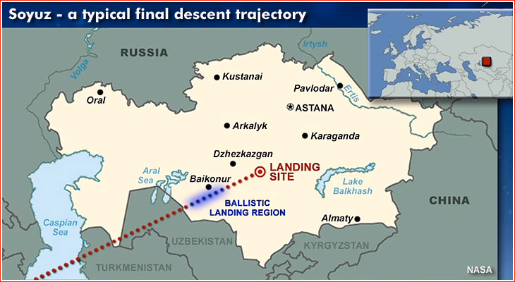
A typical final descent trajectory for the Soyuz spacecraft in Kazakhstan.
Around three minutes after exiting the plasma and around 15 minutes before landing, the capsule slows down to a speed of 900 kilometers per hour at an altitude of 13.5-12 kilometers. At that point, the cover of the parachute container is jettisoned and the parachute system begins to deploy at an altitude of around 10.5 – 9.5 kilometers.
First, two pilot parachutes with areas of 0.62 square meters and 4.5 square meters deploy, pulling out the drogue chute with an area of 24 square meters. The drogue parachute slows down the capsule from a speed of 230 meters per second to 80 meters per second (360 kilometers per hour). At this point, the main parachute with an area of 1,000 square meters opens and the braking parachute is jettisoned at an altitude of 8 – 7.5 kilometers.
When the main parachute is fully deployed, the reentry capsule enters a stable descent with a speed of around six or seven meters per second (25 kilometers per hour). Just in case, a backup parachute, half the size of the main one, is available to deploy from a separate compartment as needed.
If everything goes as planned, the flight control system initiates a series of pre-landing operations at an altitude from 5.8 to 5.6 kilometers.
First of all, the bottom heat shield of the capsule is jettisoned, revealing six solid-propellant motors, a blinking light beacon and the Kaktus-2V (“cactus”) gamma-ray altimeter. The two latter devices are immediately activated. On the sides of the capsule, external window covers are dropped.
The so-called Board of Automated Pressure Control, BARD, opens at an altitude of 5.5 kilometers to begin equalizing the pressure inside the Descent Module with the atmospheric pressure.
Also, the valves of the SIOS landing control thrusters open to drop pressurization gas and drain remaining hydrogen peroxide propellant, whose long trails of smoke are sometimes captured by tracking cameras on the search and rescue aircraft.
The Rassvet-M transmitter begins sending signals via an antenna in the parachute lines. Also, the shock absorbing system in the cosmonaut chairs is armed.
Finally, the air vessel of the main parachute is pressurized and the air is released from the backup parachute pressurization system, while the rescue system tanks, KSS, (which pump air into cosmonauts’ suits) are depressurized.
Initially, the capsule descends with its main axis under an angle of 30 degrees from the vertical axis to facilitate the cooling of its surface. At an altitude of 5.2 kilometers, and three seconds after the SIOS system drainage, the parachute’s harness disconnects from its attachment to the parachute container and instead pulls out suspension cables connected to the sides of the capsule. This switch ensures the vertical position of the spacecraft at touchdown.
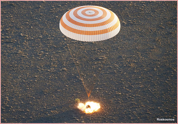
Soft-landing motors fire at touchdown.
At an altitude of eight meters, the “Posadka” (landing) signal lights up on the cosmonauts’ console and at an altitude between 1.1 and 0.8 meters from Earth, the Kaktus altimeter issues a command for the firing of the braking solid motors, DMP. The spectacular firing takes place around 0.7 meters above the surface, reducing the descent speed of the capsule to between 0 and 3 meters per second. A speed of 2 or 1.5 meters per second is considered average at the touchdown point. The structural loads on the capsule at the moment of DMP firing was quoted as 0.1 kilograms. These loads were reported to be the main reason for ruling out the reuse of the Descent Module.
In case of landing under a spare parachute, the descent speed could reach as high as 9.5 or even 10.5 meters per second, but it is still considered to be survivable by the crew.
Some additional cushioning at touchdown is provided by individual crew seats, known as Kazbek (Kazbek-UM on Soyuz TMA) equipped with custom-fitted liners for each crew member. As a last resort, the bottom of the capsule also designed to absorb the shock of a particularly bad impact.
Post-landing operations
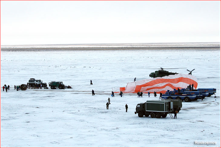
After touchdown, the cords holding the parachute are cut to prevent the capsule from being dragged by the wind, however, the craft still occasionally ends up on its side with its exhausted passengers hanging on their seat belts. In the meantime, the valves of the breathing system open into the spacecraft.
Some eight minutes after the firing of soft-landing engines, an automated command is issued to jettison the cap covering one of three housings of the ABM-279 antenna. If the capsule is on its side, one of three antennas located in the highest position also deploy. Alternatively, the same command to deploy antennas can be issued by the crew earlier. In case of a water landing, the crew has five minutes to overrule the release of the antennas at the bottom of the capsule.
Both VHF transmitters operating at 121.5 megahertz and short-wave radios, working at 8.364 and 18.060 megahertz, send their signals through the antenna helping rescue services to home in on the capsule.
If the crew exits the capsule before the arrival of rescue personnel, the cosmonauts can deploy their own ABM-281 short-wave antenna, operating at 8.364 and 18.060 megahertz.
Beginning in 2016, the signals from the autonomous navigation system, ASN, sent to mission control via two Luch data relay satellites, could also be used to pinpoint the landing site by the search and rescue team.
Because, the two out of six soft-landing motors aboard the Descent Module consist of two sections and only one of those sections fire during the nominal landing, the recovery personnel have to extract remaining live charges from the motors. Specialists then burn the solid propellant in the steppe, at a safe distance from the capsule and other members of the search personnel.
Planning the landing
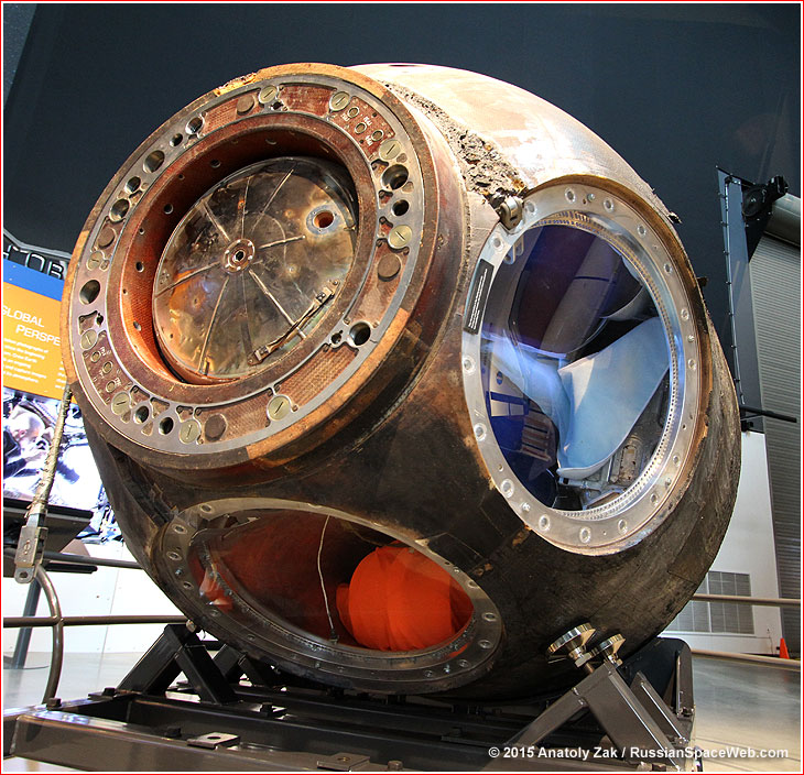
A museum copy of the Descent Module after landing.
Soyuz can land with an accuracy of only 28 kilometers, (with a probability of 0.9997), in the automated aerodynamic descent mode, AUS, relative to the center of the projected landing area.
The main reason for such a low precision is the suseptibility of the parachute landing to winds. Moreover, in case of a ballistic return, the capsule can end up as far as 600 kilometers short of the primary landing site for the aerodynamic mode.
As a result, all Soyuz landings have to be planned over a flat and open areas without any structures, rivers or even trees. A total of 13 areas currently meet all the requirements for the Soyuz landing. Ironically, all of these sites are in Kazakhstan and none of them are in Russia.
When planning Soyuz landings, engineers usually try to put the spacecraft down into the most preferable area during the first or second orbit of the day, as the spacecraft moves on the ascending arc of the orbit from south to north.
If this is impossible, they go down the list of 13 sites, according to their priority order. If nothing works, mission managers can request an orbit correction or extend the mission to ensure that the ground track of the final orbit goes over the desirable landing site.
Soyuz landing areas in Kazakhstan:
| Point |
North latitude
|
East longitude
|
| 1 |
53 degrees 00 minutes
|
49 degrees 6 minutes
|
| 2 |
53 degrees 00 minutes
|
76 degrees 18 minutes
|
| 3 |
48 degrees 06 minutes
|
75 degrees 30 minutes
|
| 4 |
42 degrees 18 minutes
|
60 degrees 30 minutes
|
| 5 |
47 degrees 06 minutes
|
58 degrees 30 minutes
|
| 6 |
49 degrees 42 minutes
|
48 degrees 00 minutes
|
| 7 |
52 degrees 00 minutes
|
48 degrees 00 minutes
|
A summary of a typical Soyuz landing:
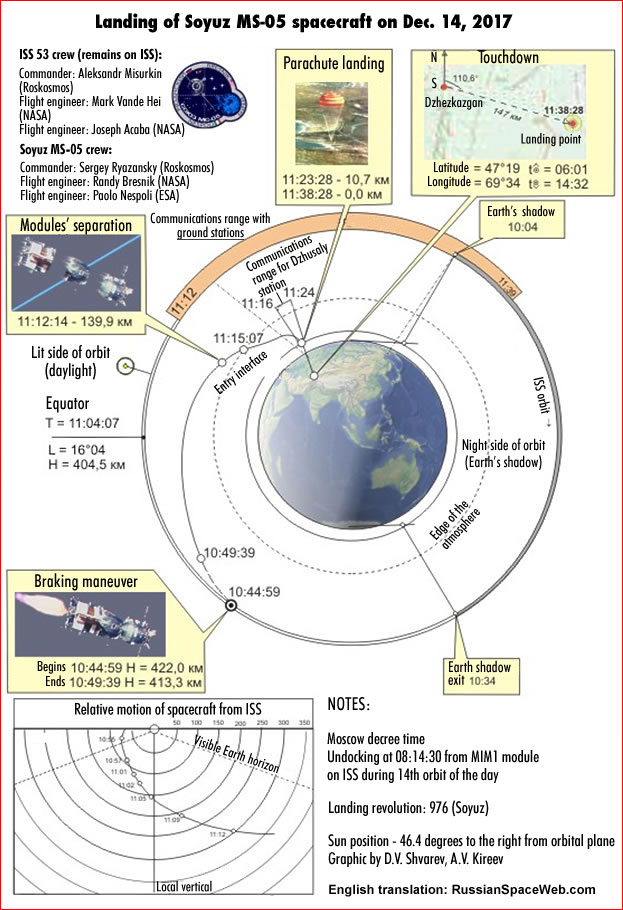
Planned landing timeline for the Soyuz MS-05 mission on Dec. 14, 2017:
| Milestone |
Moscow Time
|
Altitude, km
|
Latitude, deg. min
|
Longitude. deg, min.
|
Velocity, km/s
|
G-force
|
| Braking engine firing starts |
10:44:59
|
422.0
|
-49.05
|
315.45
|
7.352
|
0.00
|
| Braking engine firing ends |
10:49:39
|
413.3
|
-40.42
|
337.08
|
7.237
|
0.05
|
| Spacecraft sections separation |
11:12:14
|
139.9
|
+25.40
|
36.11
|
7.569
|
0.00
|
| Atmospheric entry |
11:15:07
|
099.5
|
+34.06
|
45.26
|
7.618
|
0.00
|
| Aerodynamic control starts |
11:16:38
|
080.1
|
+38.11
|
51.05
|
7.619
|
0.09
|
| Maximum G-loads |
11:21:34
|
32.9
|
+47.10
|
68.29
|
2.088
|
4.09
|
| Parachute release command |
11:23:28
|
10.7
|
+47.19
|
69.34
|
0.218
|
1.19
|
| Landing |
11:38:28
|
00.0
|
+47.19
|
69.34
|
0.000
|
1.00
|
| Main parachute opening in case of emergency ballistic descent |
11:21:19
|
10.7
|
+45.12
|
64.33
|
0.205
|
1.29
|
Estimated mass of the Soyuz TMA landing hardware:
| Main parachute, OSP |
Approximately 110 kilograms
|
| Backup parachute, ZSP |
Approximately 85 kilograms
|
| Soft-landing engines, DMP, (six) |
Approximately 60 kilograms
|
| Kazbek seats (1) |
Approximately 30 kilograms (Total: 90 kilograms)
|
Posted in Space Flight
Tagged docking, International, land, Landing, Maneuver, mechanism, module, Soyuz, Space, Station, system
Leave a comment
SpaceX’s Starhopper: Test fully successful
A gorgeous photo shows SpaceX’s Starhopper vehicle coming back down to Earth for the final time.
Starhopper, an early test prototype of SpaceX’s Mars-colonizing Starship spacecraft, flew high into the South Texas skies yesterday (Aug. 27), acing its fourth and final test jaunt. The one-minute flight took Starhopper several hundred feet up and featured a sideways translation to a landing pad a short distance away.
The new photo, which SpaceX founder and CEO Elon Musk posted on Twitter yesterday afternoon, captures Starhopper just before that touchdown. Dust kicked up by the descent billows around the vehicle, and a column of flame extends from Starhopper’s single Raptor engine down the landing pad.
The moment apparently put Musk in a contemplative mood. “One day Starship will land on the rusty sands of Mars,” he wrote in the Twitter post.
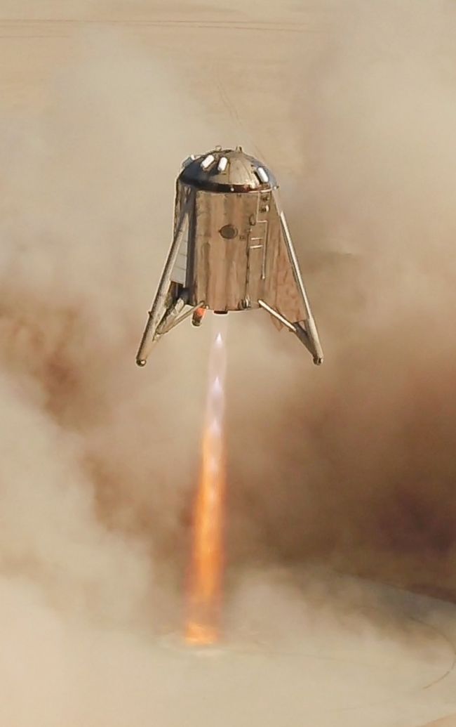
Yesterday’s flight brings that future milestone a little closer. Starhopper has proven its mettle and will now be turned into a Raptor test stand, Musk has said. The next test flights will reach Earth orbit, and they’ll be performed by advanced prototypes known as Starship Mk1 and Mk2.
Mk1 is being built at SpaceX’s facility in Boca Chica, the site that has hosted Starhopper’s forays into the sky. Mk2 is coming together on Florida’s Space Coast. The idea is to improve the design of the final 100-passenger Starship by spurring some intracompany competition, Musk has said.
Both Mk1 and Mk2 will sport at least three Raptors. The operational Starship will have six engines, and the Super Heavy rocket that will launch the spacecraft from Earth will be powered by 35 Raptors, Musk has said. (Those numbers could change, however; the billionaire entrepreneur has promised a Starship design update soon.)
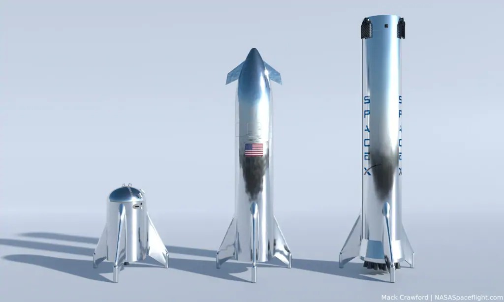
Models – From left to right: Starhopper, the test shuttle; StarShip, the 100-seat shuttle; SuperHeavy, the rocket equipped with 37 Raptor engines.
If all goes according to plan, Starship and Super Heavy could start launching satellites as early as 2021 and begin flying people just two years later. Indeed, Japanese billionaire Yusaku Maezawa has booked a Starship flight around the moon that’s currently targeted for 2023.
Starhopper’s first two hops took place in early April. On both occasions, the vehicle was tethered for safety’s sake and barely rose off the ground. Starhopper was unleashed for the first time on July 25, when the stubby prototype soared on a flight with a maximum expected altitude of 65 feet (20 meters). Yesterday’s flight had a ceiling of 150 m (about 500 feet), a limit imposed by the U.S. Federal Aviation Administration.
Hurricane Dorian in Action in these Gifs NASA and NOAA Took from Space
Updated Sept. 1, 9:40 am ET (1340 GMT): Hurricane Dorian is now a monster Category 5 storm as it nears the Abacos Islands and Grand Bahama Island.
As the storm swells closer to land, satellites operated by NASA and the National Oceanic and Atmospheric Administration (NOAA) continue to track its movement and progress. You can see some of the images from those satellite observations below, which have been shared on social media.
Related: NASA Sees Hurricane Dorian from Space Station (Video)
September 1
NOAA Satellites
✔@NOAASatellites
324 people are talking about this
August 31
NOAA Satellites
✔@NOAASatellites
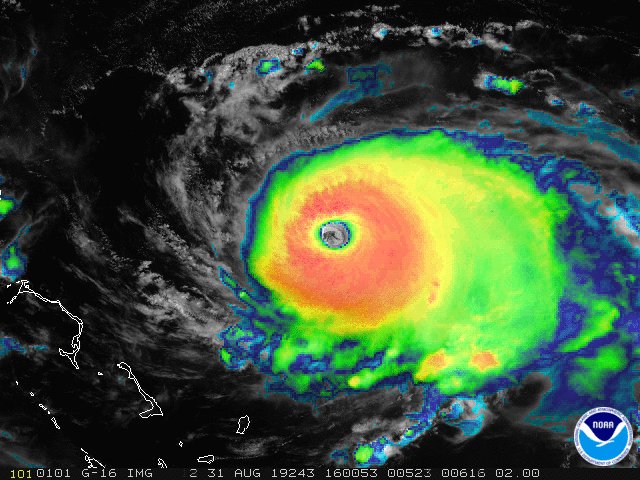
Severe #HurricaneDorian, seen in this “sandwich loop” from NOAA’s #GOESEast, is heading for the northwestern #Bahamas where the Cat. 4 storm is expected to bring life-threatening storm surge and devastating winds. Latest updates from the @NHC_Atlantic: http://nhc.noaa.gov/
390 people are talking about this
NASA
✔@NASA
Cameras outside the @Space_Station captured views of #HurricaneDorian at 11:28am ET as it churned over the Atlantic Ocean. With winds of 145 mph, the storm may approach Category 5 hurricane status, according to the National Hurricane Center. Take a look: https://go.nasa.gov/2NJz7B4


746 people are talking about this
National Hurricane Center
✔@NHC_Atlantic
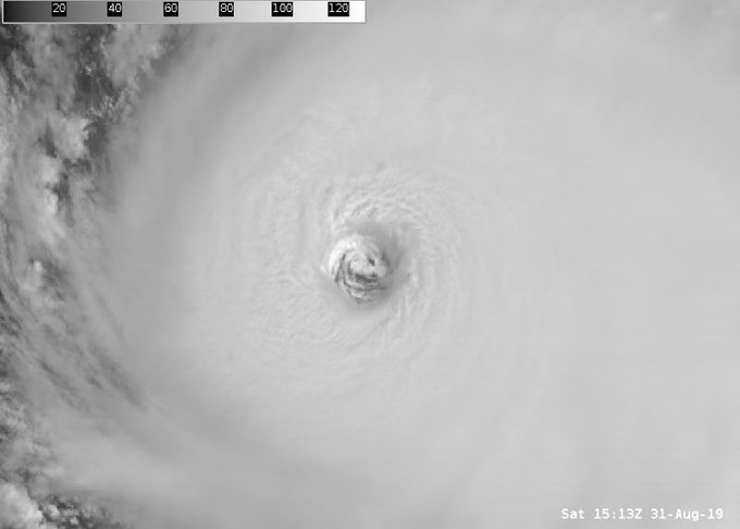
High-resolution visible imagery over the eye of #Dorian is stunning this morning. This is a special view of 30-second @NOAA high-resolution visible imagery that forecasters use. Catch the latest on this hurricane’s forecast at http://hurricanes.gov

2,153 people are talking about this
NOAA Satellites
✔@NOAASatellites
The wide eye of #HurricaneDorian is visible even from the #GOESEast perspective 22,300 miles away in space. While some fluctuations in intensity are possible, this major Cat. 4 storm is expected to remain a powerful #hurricane during the next few days. http://go.usa.gov/xVByS
545 people are talking about this
August 30
NOAA Satellites
✔@NOAASatellites
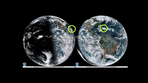
On this #FullDiskFriday, both #GOESWest and #GOESEast are keeping a close eye on extremely dangerous #HurricaneDorian from 22,300 miles in space. #Dorian is now a Cat. 3 storm with maximum sustained winds of 115 mph, according to the @NHC_Atlantic. More: http://go.usa.gov/xVB4m
64 people are talking about this
NOAA Satellites
✔@NOAASatellites
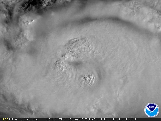
Watch as the eye of #HurricaneDorian2019 begins to form in this 1-minute visible loop from NOAA’s #GOESEast. “Dangerous Hurricane #Dorian poses a significant threat to #Florida and the northwestern #Bahamas,” according to the @NHC_Atlantic. Latest: http://go.usa.gov/xVB3K
7,188 people are talking about this
NOAA Satellites
✔@NOAASatellites
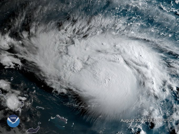
Watch as the eye of #HurricaneDorian2019 begins to form in this 1-minute visible loop from NOAA’s #GOESEast. “Dangerous Hurricane #Dorian poses a significant threat to #Florida and the northwestern #Bahamas,” according to the @NHC_Atlantic. Latest: http://go.usa.gov/xVB3K
NOAA Satellites
✔@NOAASatellites
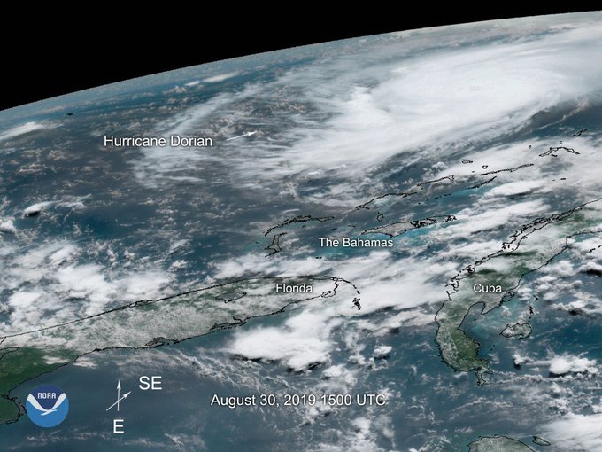
Major #HurricaneDorian, seen here by NOAA’s #GOESWest, is now an extremely dangerous Cat. 3 storm. #Dorian is expected to strengthen and “poses a significant threat to #Florida and the northwestern #Bahamas,” according to the @NHC_Atlantic. More: http://go.usa.gov/xVBTg
238 people are talking about this
NASA SPoRT
✔@NASA_SPoRT
Evening RT: Using satellite imagery from the @NASARain Constellation to diagnose the evolution of cloud and precipitation structure in Hurricane #Dorian >>https://go.nasa.gov/2MLO5a2


See NASA SPoRT’s other Tweets
Intl. Space Station
✔@Space_Station
Cameras outside the space station captured these views of rapidly intensifying #HurricaneDorian at 12:18pm ET on August 30 as it churned over the Atlantic Ocean. For more on NASA’s coverage of #Dorian, visit: http://nasa.gov/press-release/nasa-to-provide-coverage-of-hurricane-dorian ….


2,445 people are talking about this
NOAA Satellites
✔@NOAASatellites
Take a look at all that lightning! The Geostationary Lightning Mapper aboard NOAA’s #GOESEast captured this view of all the lightning associated with #HurricaneDorian2019 in the morning hours of Aug. 30, 2019. Follow the storm’s path here: http://go.usa.gov/xVZu9
602 people are talking about this
NOAA Satellites
✔@NOAASatellites
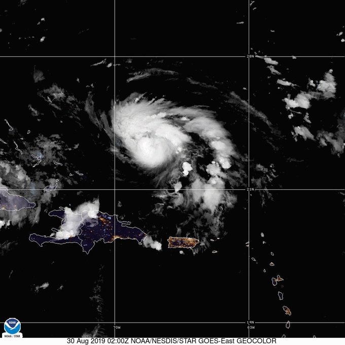
Hurricane #Dorian, seen here by NOAA’s #GOESEast, is now a Cat. 2 storm with maximum sustained winds of 110 mph. A #HurricaneWatch is now in effect for the northwestern #Bahamas as the storm slowly churns across the western #Atlantic. More: http://go.usa.gov/xVZMX
98 people are talking about this
NASA Earth
✔@NASAEarth
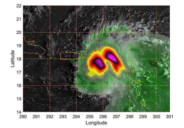
TEMPEST-D, a weather-observing CubeSat, used its miniaturized radio-wave-based instrument to see through the clouds, showing areas with strong rain and moisture being pulled into the storm.
Green = Moisture spiraling into the storm’s center
Yellow to Pink = Intense rainfall

NASA Earth
✔@NASAEarth

76 people are talking about this
NOAA Satellites
✔@NOAASatellites
Hurricane #Dorian, seen here by NOAA’s #GOESEast, is now a Cat. 2 storm with maximum sustained winds of 110 mph. A #HurricaneWatch is now in effect for the northwestern #Bahamas as the storm slowly churns across the western #Atlantic. More: http://go.usa.gov/xVZMX
98 people are talking about this
August 29
Intl. Space Station
✔@Space_Station
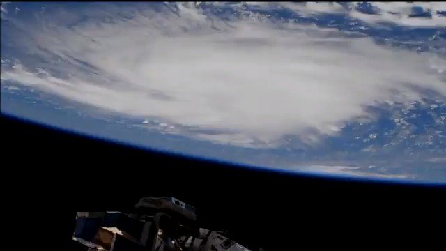
A camera outside the station captured views of Hurricane Dorian at 1:05pm ET today as it churned over the Atlantic Ocean north of Puerto Rico.
2,489 people are talking about this
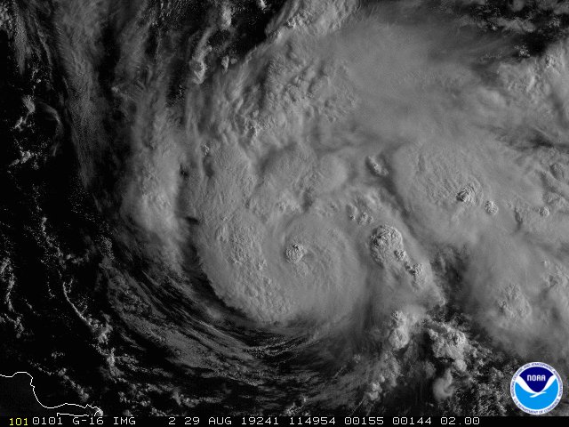
NOAA Satellites PA@NOAASatellitePANEW: This morning’s latest visible satellite animation from #GOES16 of #HurricaneDorian as it moves away from #PuertoRico and the #VI into the open waters of the Atlantic. Updates: @NHC_Atlantic

171 people are talking about this
August 28
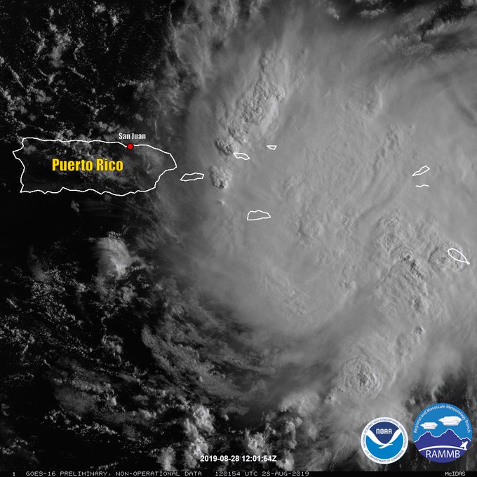
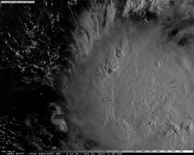
NOAA Satellites PA@NOAASatellitePAThis visible satellite animation from NOAA’s #GOES16 shows #TropicalStormDorian moving closer to the #VirginIslands and #PuertoRico this morning. Get the latest @NHC_Atlantic update here: https://www.nhc.noaa.gov/
273 people are talking about this
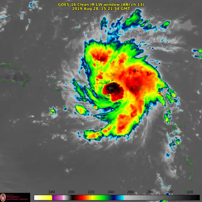
UW-Madison CIMSS@UWCIMSS#GOESEast meso-sector is tracking #TropicalStormDorian. View 1-minute imagery of TS #Dorian via multiple #GOES16 bands HT @UW_AOS at http://www.aos.wisc.edu/weather/wx_obs/GOES16_meso2.html …

21 people are talking about this
NASA SPoRT
✔@NASA_SPoRT
Latest look at Hurricane #Dorian from @NOAA‘s GOES16. For official information stay tuned to @NHC_Atlantic and local @NWS WFOs.
33 people are talking about this
NOAA Satellites
✔@NOAASatellites
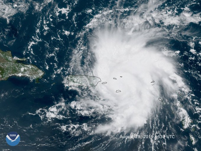
Earlier this afternoon #Dorian strengthened to a Cat. 1 #hurricane with maximum sustained winds of 75 mph. NOAA’s #GOESEast spotted the storm moving toward the #VirginIslands, where hurricane warnings are now in effect. Follow the storm’s path here: http://go.usa.gov/xVWkT
128 people are talking about this
August 27
NOAA Satellites
✔@NOAASatellites
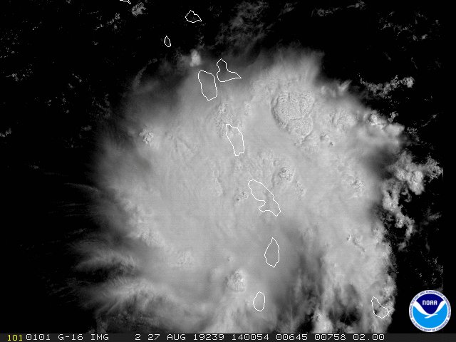
Tropical Storm #Dorian, seen in this view from NOAA’s #GOESEast, moved over the Lesser Antilles this morning. While uncertainty remains high, the @NHC_Atlantic says wind and rain from this system could impact the Bahamas and Florida later this week. More: http://go.usa.gov/xVD3A
46 people are talking about this
August 26
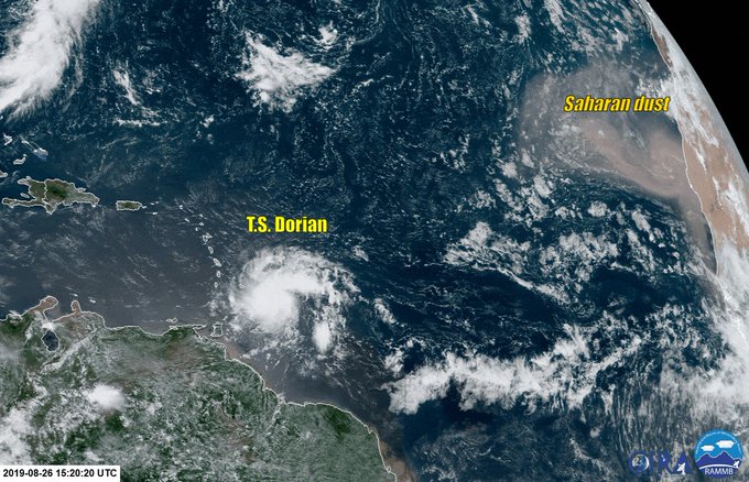
NOAA Satellites PA@NOAASatellitePAAs #TropicalStorm #Dorian spins in the Atlantic, NOAA’s #GOES16 is keeping an eye on it. You can also see the #dust coming off the #SaharaDesert at the top right. Here’s the latest #tropical update: https://www.nhc.noaa.gov/
113 people are talking about this
NOAA Satellites PA@NOAASatellitePA
Hubble Telescope: How it Works?
Orbiting high above the Earth, the Hubble Space Telescope has a clear view of the universe free from the blurring and absorbing effects of the atmosphere. In addition to observing visible and near-infrared light, Hubble detects ultraviolet light, which is absorbed by the atmosphere and visible only from space. The telescope has beamed hundreds of thousands of celestial images back to Earth during its time in space.
Hubble is a Cassegrain reflector telescope. Light from celestial objects travels down a tube, is collected by a bowl-like, inwardly curved primary mirror and reflected toward a smaller, dome-shaped, outwardly curved secondary mirror. The secondary mirror bounces the light back to the primary mirror and through a hole in its center. The light is focused on a small area called the focal plane, where it is picked up by its various science instruments.
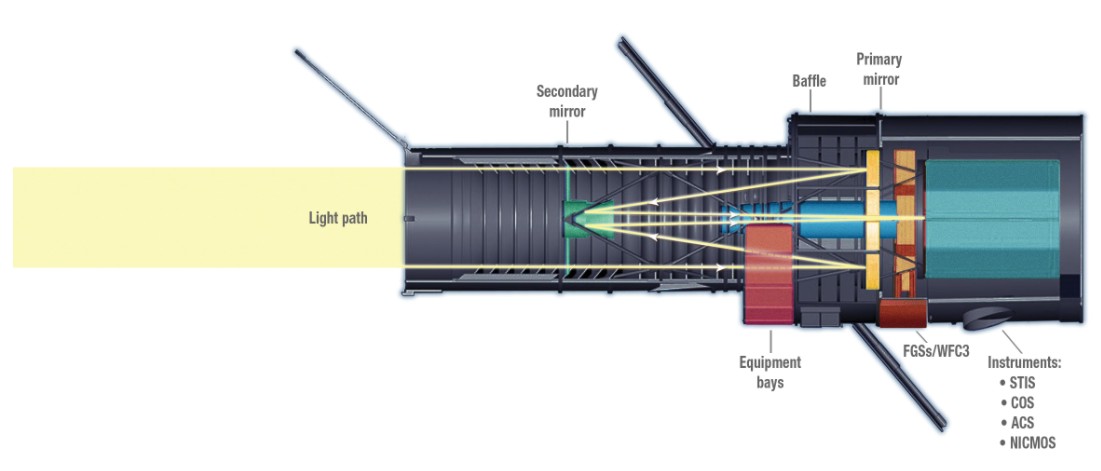
Hubble’s 1,825 pound, 7.8-foot (2.4-meter) diameter primary mirror collects light from its astronomical target and reflex it to a 12-inch (0.3-meter) diameter secondary mirror located in the optical tube. This secondary mirror then reflects the light through a hole in the primary mirror to form an image at the telescope’s focal plane. There it is intercepted by pick-off mirrors that pass it into the scientific instruments. Hubble’s mirrors are made of ultra-low expansion glass kept at a “room temperature” of about 70°F (21°C) to avoid warping. The reflecting services are coated with a 3/1000,000-inch layer of pure aluminum and protected by a 1/1000,000-inch layer of magnesium fluoride that also makes the mirror is more reflective to ultraviolet light.
Hubble’s science instruments, the astronomer’s eyes to the universe, work together or individually to provide the observations. Each instrument is designed to examine the universe in a different way. Hubble holds two main varieties of instruments: cameras, which capture Hubble’s famed images, and spectrographs, which break light into colors for analysis.
Hubble’s current suite of instruments includes the Wide Field Camera 3 (WFC3), Cosmic Origins Spectrograph (COS), Advanced Camera for Surveys (ACS), Space Telescope Imaging Spectrograph (STIS) and Fine Guidance Sensors (FGS).
These are not the only instruments that have flown aboard Hubble. The telescope was designed to be visited periodically by astronauts, who brought new instruments and technology, and made repairs from December 1993 to May 2009.
After launch in April 1990, NASA discovered that the primary mirror was flawed. The flaw was tiny, only about 1/50th
the width of a human hair, but significant enough to distort Hubble’s vision. During Servicing Mission 1 in December of 1993, astronauts added corrective optics to compensate for the flaw. The optics acted like eyeglasses to correct Hubble’s vision.
Spacecraft systems
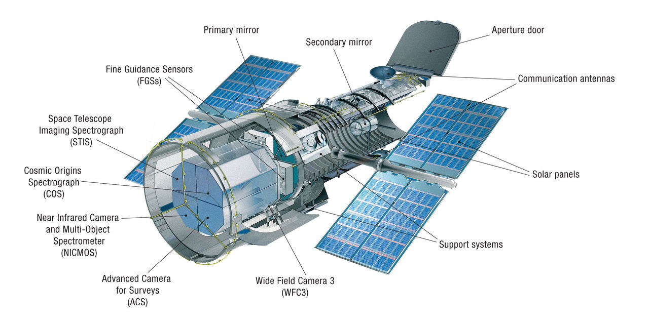
Hubble’s Control and Support Systems and Instruments Diagram
The forward shell houses the telescope’s optical assembly. In the middle of the telescope are the reaction wheels and the bays that house the observatory’s control electronics. The aft shroud houses the scientific instruments, gyroscopes, and star trackers.
Hubble is operated by commands from the ground. Several spacecraft systems are in place to keep Hubble functioning smoothly.
Communications antennas
Hubble performs in response to detailed instructions from people on the ground. The antennas allow technicians to communicate with the telescope, telling it what to do and when to do it. Four antennas receive and send information to a set of satellites, which in turn communicate with Earth.
Solar arrays
Hubble is powered by sunlight. Each wing-like array has solar cells that convert the Sun’s energy into electricity. Some of that electricity runs the telescope, some is stored in onboard batteries for the periods when Hubble is in Earth’s shadow.
Computers and automation
Several computers and microprocessors reside in Hubble’s body and in each science instrument. There are two main computers. One talks to the instruments, sends commands and other information, and transmits data; the other handles pointing control, gyroscopes and other system-wide functions.
Thermal protection
Hubble has blanket of multilayered insulation, which protects the telescope from temperature extremes.
Pointing system
Hubble uses a combination of gyroscopes, reaction wheels and Fine Guidance Sensors to orient itself.
Science of Hubble
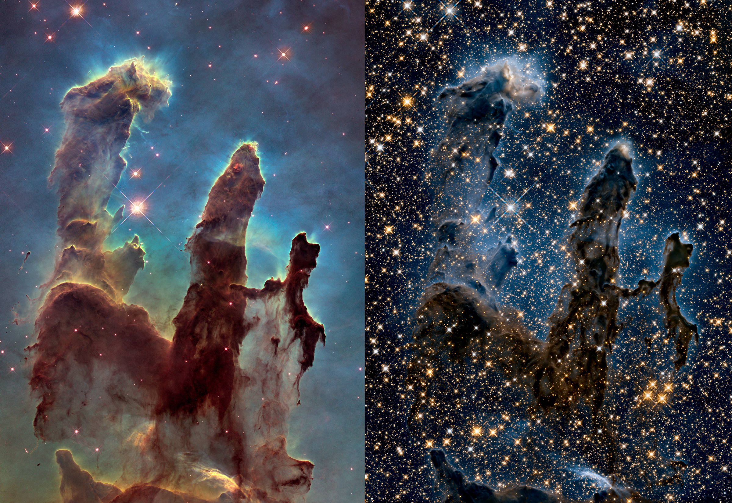
Pillars of Creation
Hubble WFC3 images of M16 in visible light (left) and near-infrared light (right).
Hubble is one of NASA’s most successful and long-lasting science missions. It has beamed hundreds of thousands of images back to Earth, shedding light on many of the great mysteries of astronomy.
Among its many discoveries, Hubble has revealed the age of the universe to be about 13.8 billion years, much more accurate than the old range of anywhere from 10 to 20 billion years. Hubble played a key role in the discovery of dark energy, a mysterious force that causes the expansion of the universe to accelerate.
Hubble has shown scientists galaxies in all stages of evolution, including galaxies that were around when the universe was still young, helping them understand how galaxies form. It found protoplanetary disks, clumps of gas and dust around young stars that likely function as birthing grounds for new planets. It discovered that gamma-ray bursts — strange, incredibly powerful explosions of energy — can occur in far-distant galaxies when massive stars collapse. And these are only a handful of its many continuing contributions to astronomy.
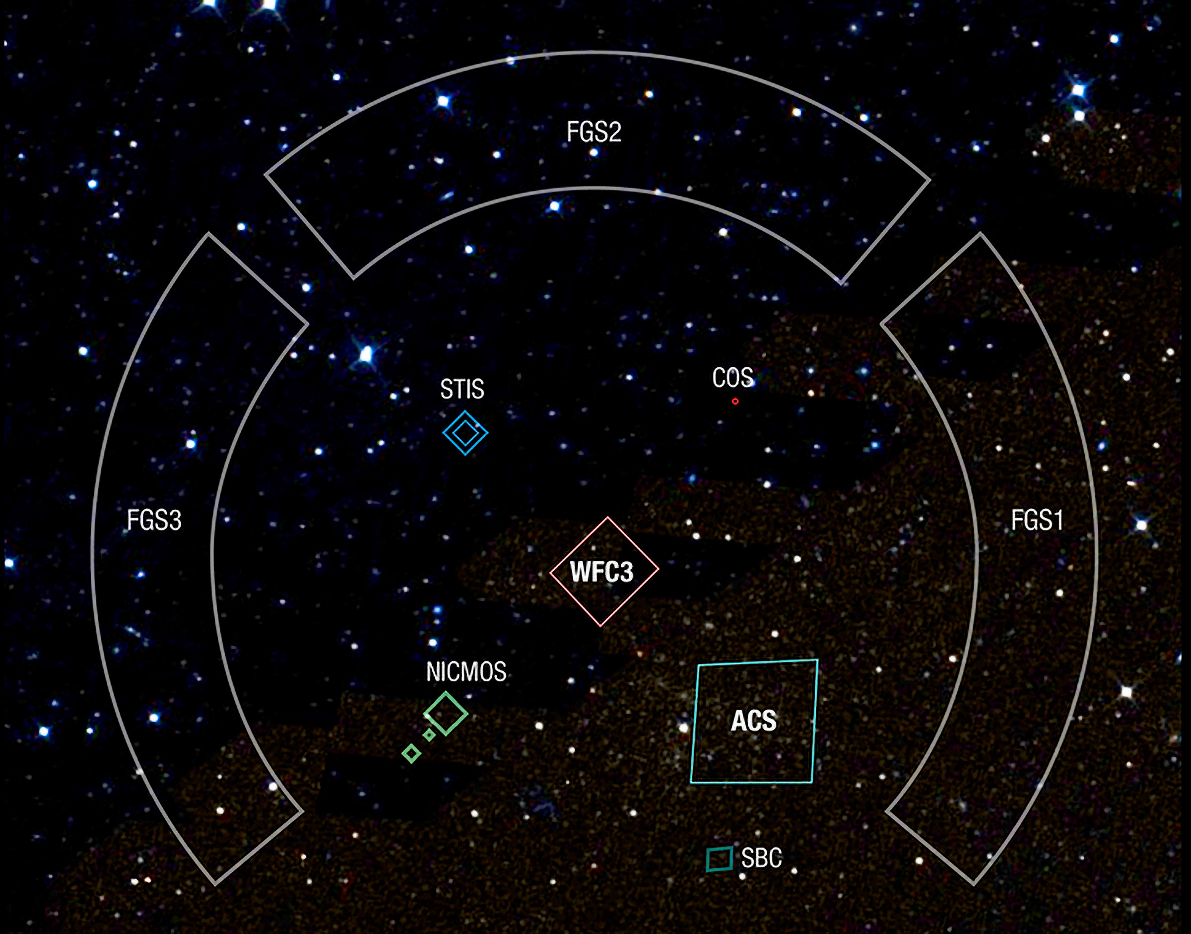
The Field of View (FOV) “footprints” of Hubble’s Instruments
Instruments include the fine guidance sensors (FGSs), Near Infrared Camera and Multi-Object Spectrometer (NICMOS), Space Telescope Imaging Spectrograph (STIS), Cosmic Origins Spectrograph (COS), Wide Field Camera 3 (WFC3), and Advanced Camera for Surveys (ACS), which includes the Solar Blind Channel (SBC).
The telescope is an instrument for the entire astronomical community. Any astronomer in the world can submit a proposal and request time on the telescope — alone or in coordination with other observatories in space and on the ground — as well as for support to make use of Hubble’s extensive data archives. Astronomers compete for time to use Hubble.
More scientists want to use the telescope than time allows, so a review committee of astronomy experts has to pick out the best proposals from the bunch. To avoid bias, the competition process is double-blind. This means that not only are proposers unaware of the identity of the reviewers, but the reviewers are also not aware of the identities of proposers.
The winning proposals are the ones that make the best use of the telescope’s capabilities while addressing pressing astronomical questions. Each year around 1,000 proposals are reviewed and approximately 200 are selected, for a total of about 20,000 individual observations.
WHAT’S ON BOARD
Hubble was designed to hold six science instruments, each observing the universe in a unique way. The telescope has cameras, which capture Hubble’s famed images, and spectrographs, which break light into colors for analysis. The current suite of instruments is listed below.
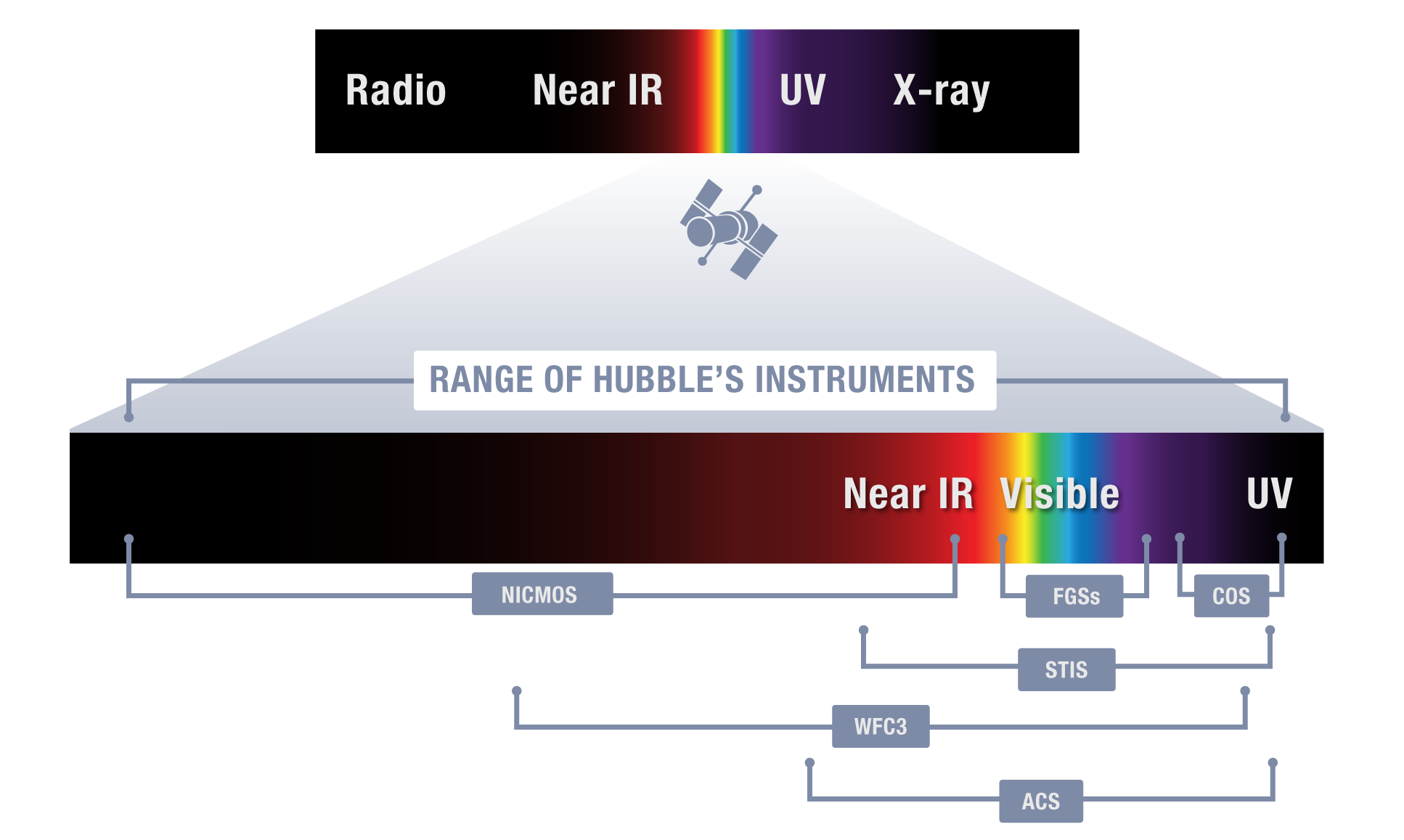
Hubble’s instruments collectively observe wavelengths (measured in nanometers) from ultraviolet through infrared. Each instrument was designed to operate in a particular wavelength range and function as an imaging camera or a spectrometer, though some instruments do both. The Fine Guidance Sensors (FGSs) not only help the telescope stay locked on target, but can be used as science instruments to accurately determine the relative position of stars.
Wide Field Camera 3
Wide Field Camera 3 (WFC3) expanded Hubble’s reach by giving the telescope greater access to ultraviolet, visible and infrared wavelengths of light. With its high resolution and wide field of view, WFC3 has become the telescope’s workhorse camera, responsible for many of Hubble’s spectacular pictures. It has imaged everything from nearby star formation to galaxies in the very distant universe.
Cosmic Origins Spectrograph
The Cosmic Origins Spectrograph (COS) breaks ultraviolet radiation into components that can be studied in detail. COS is best at studying points of light, like stars or quasars (distant galaxies emitting tremendous amounts of light from their central regions). It has been used to study galaxy evolution, the formation of planets and the rise of the elements needed for life.
Advanced Camera for Surveys
The Advanced Camera for Surveys (ACS) conducts surveys of the universe. It is responsible for many of Hubble’s most impressive visible-light images of deep space. With its wide field of view, sharp image quality, and high sensitivity, ACS helps map the distribution of dark matter, detects the most distant objects in the universe, searches for massive planets and studies the evolution of clusters of galaxies.
Space Telescope Imaging Spectrograph
The Space Telescope Imaging Spectrograph (STIS) combines a camera with a spectrograph, which provides a “fingerprint” of a celestial object’s temperature, chemical composition, density and motion. STIS also reveals changes in the evolving universe and leads the way in the field of high-contrast imaging. The versatile instrument is sensitive to a wide range of wavelengths of light, from ultraviolet through the optical and into the near-infrared. STIS studies black holes, monster stars, and the intergalactic medium, and analyzes the atmospheres of worlds around other stars.
Near Infrared Camera and Multi-Object Spectrometer
The Near Infrared Camera and Multi-Object Spectrometer (NICMOS) is sensitive to infrared light, which is perceived by humans as heat. Infrared light reveals details about distant galaxies, planets and solar systems and star formation that are not available in visible light. It observes objects hidden by interstellar dust, such as site of stellar formation. The instrument sports three cameras — each with different fields of view. NICMOS operated from 1997 to 1999, and from 2002 to 2008.
Fine Guidance Sensors
Hubble’s three Fine Guidance Sensors (FGS) — its targeting cameras — are devices that lock onto guide stars and keep Hubble pointed in the correct direction. Two of the sensors point the telescope at an astronomical target and then hold that target in a scientific instrument’s field of view. The third sensor is available to perform scientific observations, precisely measuring the distance between stars and their relative motions.

This diagram shows the locations of Hubble’s instruments inside the telescope. The instruments are located in containers that make them easy to remove and replace. Credit: NASA, ESA.
Additional Telescope Features
Primary mirror
Hubble’s primary mirror is 7.8-feet (2.4-meters) in diameter. It is made of a special glass coated with aluminum and a compound that reflects ultraviolet light. It collects light from the telescope’s targets and reflects it to the secondary mirror.
Secondary mirror
Like the primary mirror, Hubble’s secondary mirror is made of special glass coated with aluminum and a compound to reflect ultraviolet light. It is 12 inches (30.5 centimeters) in diameter and reflects the light back through a hole in the primary mirror and into the instruments.
Aperture door
Hubble’s aperture door can close, if necessary, to prevent light from the Sun from entering and potentially damaging the telescope or its instruments.
Communication antennas
Digital images and spectra stored in Hubble’s solid-state recorders are converted to radio waves and then beamed through one of the spacecraft’s high-gain antennas (HGAs) to a NASA communications satellite, which relays them to the ground. Because the HGAs would extend off the page above and below the spacecraft image, they are shown here pressed against the side of the telescope in their “berthed positions.” This is how they were configured at launch.
Solar panels
Hubble’s current set of rigid solar panels use gallium-arsenide photovoltaic cells that produce enough power for all the science instruments to operate simultaneously. The first and second sets were larger, flexible panels, but produced less power.
Support systems
Essential support systems such as computers, batteries, gyroscopes, reaction wheels, and electronics are contained in these areas.
[smartslider3 slider=”2″]
Airbus Unveils New ‘Bird of Prey’ Concept Plane
Airbus has unveiled a bird-like concept for a hybrid-electric airliner that aims to show the potential of using biomimicry in aviation design.
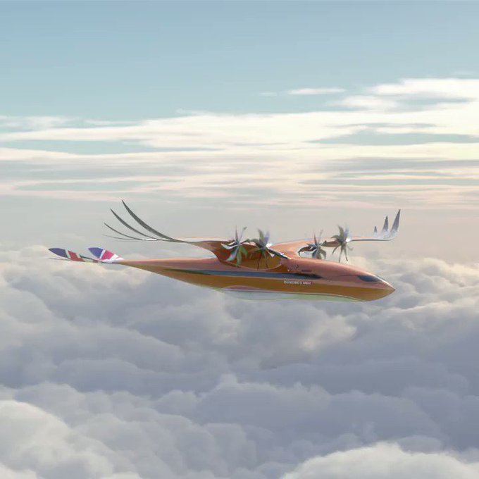
Inspired by the “efficient mechanics” of birds, Airbus’ Bird of Prey conceptual aircraft features wing and tail structures with individually controlled feather-like tips, which help with control while minimising drag.
The concept also boasts a smooth wing root – the point where the wing joins the fuselage – designed to imitate the graceful, aerodynamic arch of an eagle or falcon.
The feathered tips of the plane’s tail are decorated with the pattern of a union jack, which contrasts with its orange body and more subtly coloured blue, white and gold wings.
While not intended to represent an actual aircraft, the Bird of Prey concept is based on realistic ideas. Its designers are aiming to provide an insight into what the future of aviation could look like if designers harnessed the potential of biomimicry – design inspired by nature.
 The ‘#BirdOfPrey’ is taking wing! This sleek new concept takes inspiration from eagles to create a hybrid-electric design with individually controlled feathered wings. We’re always looking for pioneering new ideas – what would your aircraft be inspired by? https://fly.airbus.com/2xSKQ7c
“Our Bird of Prey is designed to be an inspiration to young people and create a ‘wow’ factor that will help them consider an exciting career in the crucially important aerospace sector,” said Martin Aston, a senior manager at Airbus.
“One of the priorities for the entire industry is how to make aviation more sustainable – making flying cleaner, greener and quieter than ever before,” he continued.
“We know from our work on the A350 XWB passenger jet that through biomimicry, nature has some of the best lessons we can learn about design,” added Aston.
The plane would be able to accommodate up to 80 passengers, and would have a range of 1,500 kilometres.
Thanks to its hybrid-electric propulsion system the Bird of Prey would burn 30 to 50 per cent less fuel than todays airliners do, providing optimal low-speed performance while working to reduce environmental emissions.
This electric system would power propellers made of carbon fibre, and would also produce less noise than typical aircrafts.
Around the same time, in February, Airbus announced it was ceasing production of the A380 – the world’s largest passenger aircraft. We spoke to Paul Priestman, who designed the superjumbo’s first interior, about the plane’s design legacy.
AlbatrossOne Airbus, Revolutionising Aircraft Wing Design
Airbus has commenced testing of a scale model demonstrator intended to explore the benefits of hinged wing-tips to alleviate gust loads and consequently reduce aircraft structural weight.
While locking hinged wing-tips – such as those on the new Boeing 777X – are designed to reconcile high aspect ratio wings with the constraints of airport gates, the AlbatrossOne demonstrator is designed to examine the advantages of allowing them to continue moving during flight.
AlbatrossOne is named for the gliding marine bird which travels long distances using wings which lock at the bird’s shoulder for dynamic soaring but which unlock when required for propulsion, manoeuvring or turbulence response.
The aircraft model, resembling an A321, features analogous hinges allowing the outer 25% of the wing to move freely.
Airbus says the semi-aeroelastic hinge concept – neither purely active nor purely passive – centres on a lock which would permit the sudden release in response to a gust.
Executive vice-president of engineering Jean-Brice Dumont, speaking at the airframer’s Innovation Days event in Toulouse, said the AlbatrossOne project “shows how nature can inspire us”.
The albatross has an aspect ratio of up to 18:1, around twice that of the A321. Greater span reduces induced drag, which represents a high proportion of overall drag.
First test flights with AlbatrossOne were conducted in the last few weeks, he says. The model was developed over 20 months by Airbus’s UK facility in Filton – the airframer describes it as the “first Filton aircraft since Concorde”.
It has been constructed from materials including carbonfibre and glassfibre reinforce polymers, as well as components from additive layer manufacturing, and plywood.
Dumont says that, during a wind gust, the wing of a conventional aircraft transmits high levels of load to the fuselage, which requires the wing box to be heavily reinforced.
But detecting the gust and allowing the wing-tip to flex alleviates these loads and means the wing structure can be considerably lighter.
Dumont acknowledges that the hinged wing-tip “adds complexity” but believes the potential lighter structures and fuel savings would outweigh this disadvantage.
Airbus already uses load-alleviation strategies on its aircraft through the activation of ailerons and spoilers.
Initial flights of AlbatrossOne have focused on the stability of the aircraft with the wing-tips locked and completely unlocked, to check there are no adverse effects.
Dumont says the next step is to conduct further tests to combine the two modes, allowing the wing-tips to unlock during flight and to examine the transition.
Future development would require an actuator to be fitted in order for the aircraft to revert to locked wings, and to allow the wing-tips to fold during gate docking.
Dumont says the research will look at the optimum size of the hinged portion. He indicates that Airbus would eventually work towards a full-size demonstrator, but stresses that such a development is several years away.
“The technologies are basically available,” he says. “The question is how they match on board an aircraft.”
Airbus revealed in a research paper last October that it was modelling the behaviour of semi-aeroelastic wing-tips to study whether the tips – if left unlocked – could contact the ground during landing.
Preliminary conclusions from the modelling, based on a short-range aircraft with a 45m span and 4.5m folding tips, indicate that aerodynamic stiffness and damping effects would prevent ground contact across a variety of scenarios for descent rate, bouncing, and rolling.
“There may be cases where contact is possible,” says the paper. “However, even in such a scenario this study suggests that countermeasures such as stoppers would likely not have to be very substantial.”
Analysis is also being undertaken as to whether the wing-tips could exhibit life limit oscillations, although the paper states that the AlbatrossOne test aircraft has been designed with a stiff wing to avoid wing-tip flapping and wing-bend coupling.
Skyrora successfully flight tests 3D printed rocket
SCOTTISH space company Skyrora has successfully carried out testing on a fully 3D-printed, commercial rocket engine for the first time ever in the UK.
The Edinburgh-based firm used its base in Cornwall to carry out engine checks on its XL rocket, the firm’s main orbital launch vehicle.
The engine boasts stop-start technology, meaning Skyrora’s rocket can deliver satellites to different orbits.
Vladimir Levykin, CEO at Skyrora, said, “It’s always exciting to reach testing stage and even more so for our XL rocket.
“Not only is it our main orbital launch vehicle but this is the first time a commercial, fully 3D-printed bi-liquid rocket engine has been tested in the UK.
“Naturally we’re delighted that the tests have gone so well over both testing days and it’s a testament to the dedicated work of the team that we’ve reached this stage so smoothly.
The engine’s 3D-printed technology allows cooling channels to be embedded into the walls of the combustion chamber. According to Skyrora this means the engine requires fewer parts. making it more straightforward to assemble, boosting reliability and cost-effectiveness.
Since the birth of the Space Age, the high cost and long lead times associated with launching satellites into orbit have represented a major barrier to the commercialization and exploration of space. As a result, the sector has been occupied mostly by large companies and government-backed organizations. However, in recent years the rapid growth and evolution of nano- and microsatellite technology has given birth to a burgeoning industry and led to the establishment of almost 70 companies and organizations dedicated to the development of low-cost launch platforms.
Rocket-developer Skyrora in Edinburgh, Scotland, was founded in 2017. The company is set to begin its engine testing program this year, having 3D printed its first engines and began production of its proprietary oxidizer propellant. Daniel Smith, director of business development at Skyrora, says, “Our launch vehicle is suitable for use in the UK thanks to a number of factors, including our choice of propellant combination, which has storability benefits and removes any requirement to de-tank during weather delays.”
According to Smith, the team is adopting a step-by-step approach to development and has already begun to test systems and de-risk the suborbital vehicles. They will then move on to testing the orbital vehicle to coincide with the first UK spaceport being operational.

Skyrora’s rocket runs on Hydrogen Peroxide and Kerosene (Image: Skyrora)
“Our strategy is to combine proven and new technology to produce a launcher that is reliable and cost-effective. There’s no need to reinvent the wheel across the board,” says Smith.
Skyrora’s rocket engine is based on technology from UK programs from the 1950s and 1960s, such as Skylark and Black Arrow, and will run off high-test peroxide (HTP) and kerosene.
Smith says that the key to successful development for Skyrora is to “take the relevant elements of what worked so well before and use modern, advanced manufacturing techniques to improve the build efficiency and bring the cost of mass production down”
For example, the engineering team is planning to use 3D printing to make parts of its engines “where it makes sense to”, says Smith.
Testing Flexibility
Elsewhere, Calverton, New York-based startup Launcher is also in the process of building an orbital launch vehicle, capable of delivering a 300kg (660 lb) payload to a 200km orbit. The company is developing a low-cost 3D-printed engine with a staged combustion cycle.
As Max Haot, CEO of Launcher, explains, the company is following a three-phase plan to develop the final 22,000 lbf (98,000N), LOX/RP-1 (liquid oxygen/rocket propellant 1) staged combustion engine, called Engine-2 (E-2).
The first phase, which has run for the past 12 months, has focused on the development and testing of Engine-1 (E-1), a 500 lbf (2,220N), LOX/RP-1 pressure-fed, 3D-printed engine made up of three Inconel 718 parts and an augmented spark igniter. E-1 is a 1/40th subscale version of the flight engine, which will be used to test the company’s regenerative cooling design in advance of the larger E-2 chamber. “E-1 is also being used to build our test site, electronics, software, test stand development, and operation skills and 3D-printing experience. We are nearing the end of this test campaign,” says Haot.
Phase 2 will run for the next three years to develop E-2. According to Haot, LOX pump development is currently in progress, with the goal being to test the turbo pump assembly “by the end of 2019, with the engine firing by the end of 2020”.
Phase 3, which will only start following a successful E-2 test campaign, will consist of the scaling up of the team and funding to develop the full launch system. The first test flights are expected to be in 2024 and 2025, with commercial operation expected by the end of 2026.
Haot says, “We believe the key is 3D printing the engine to optimize the size and performance to handle 22,000 lbf. We need to ensure that we can take advantage of 3D printing for low-cost and flexible iterations without tooling.”
For Haot, the fact that the Launcher team has its own test site and test stand, developed end-to-end, is critical to testing flexibility and quick iterations. For example, he reveals that the team does not use off-the-shelf DAQ hardware or software.
“Everything is custom electronics and software, so we have full control and so we are close to an actual flight architecture for software and electronics,” he says.
“Keeping the team small and staying a startup, we are able to test E-1 every week with just three people on-site. We are staying focused and small until we complete our E-2 engine development.”
Low-cost projects in aerospace are not restricted to providing cheaper access to space. The Space Drone project is aiming to reduce the cost of satellite maintenance. Arie Halsband, CEO of Effective Space, believes a number of satellites that “required hundreds of millions of dollars to place into orbit” are made redundant each year, not because they are fundamentally broken, but “because their fuel reserves are depleted”.
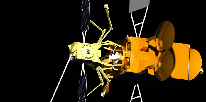
The Space Drone will act as an external jet pack for satellites
Last-Mile Logistics
In an effort to address this challenge, the company plans to deploy and operate a fleet of small spacecraft capable of delivering, positioning, maintaining and monitoring satellites. According to Halsband, in January this year Effective Space signed a multi-year contract worth more than US$100m with a leading regional satellite operator for a mission that will start in 2020 and includes the “life extension of two communication satellites”.
Each spacecraft will weigh around 400kg (880 lb) and measure about 1m3 (35ft3) in size. The Space Drone is propelled by what is described as an external jet pack with a proprietary, rideshare compatible, all-electric, small yet capable platform design. “It safely and accurately performs rendezvous and docking with the host satellite with a patent-pending non-intrusive docking arms system. Its electric propulsion also allows for up to 15 years of service,” Halsband says.
Development of the Space Drone began in 2014, and by December 2017, the spacecraft had achieved hundreds of successful docking tests. This first phase of testing used hardware-in-the-loop testing at technology group GMV’s facility in Madrid, Spain, to emulate zero-gravity dynamic conditions. The GMV facility is also used for ESA ground tests of a spacecraft’s docking equipment and the procedures it conducts with the International Space Station.
Engineers at GMV will also verify the rendezvous and docking system, test the sensor engineering models, and check the onboard computers that run the guidance, navigation and control software, as well as the docking arms system, ensuring that the spacecraft are fully validated for launch.
“No satellite operator would pay for a servicing spacecraft if the cost were the same as buying and launching a replacement satellite. To prove the business case for in-orbit servicing, it was therefore vital to create a viable spacecraft that could be built, launched and operated for at least half of a normal satellite’s price,” says Halsband.
A notable measure the company has employed to reduce cost and testing timescales is to pursue a ‘minimum viable’ product approach. Unlike previous attempts, and “certain other current attempts” to provide satellite servicing capabilities, the Space Drone’s design strictly uses GEO station-keeping and attitude-control maneuvers.
“Relying on an all-electric solution, deployable mechanisms and a simple and safe docking system, all contribute to the simplicity and the robustness of the platform,” Halsband says.
Revolutionary Advances
The furthest forward in the small satellite launch sector is Huntington Beach, California-based startup Rocket Lab. The company’s Electron rocket is designed with a focus on delivering a high number of launches. After a successful launch from New Zealand in January this year, it is the only dedicated small satellite launch provider to have deployed satellites to orbit.
Peter Beck, CEO at Rocket Lab, says, “Until now, small satellites have been a secondary payload, hitchhiking on a rocket with larger satellites that dictate the orbit and launch schedule, which is often prone to delays.
“We provide a service dedicated solely to small satellites, giving our customers flexibility over when they launch and the orbit they want to reach.”
According to Beck, the Electron launch vehicle will feature the first electric pump-fed rocket engines in the world. All components for the Electron are designed and made in-house by the company, which also operates its own launch site on the Mahia Peninsula in New Zealand.
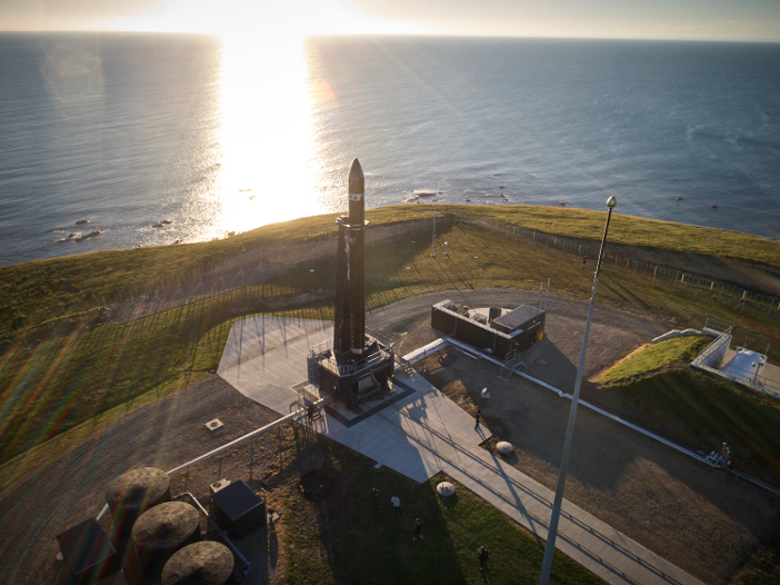
Rocket Lab has the world’s first private orbital launch site in New Zealand
Rocket Lab has adopted several strategies to minimize costs and the time it takes to make rockets. For example, the electric propellant pumps reduce mass and its Rutherford engines are 3D printed in just 24 hours.
“We have used both commercial and in-house simulation tools to develop everything in the launch vehicle, including guidance and propulsion,” says Beck.
“To test launch vehicles, we follow all the traditional military and NASA standards. Rocket Lab is test heavy – we build hardware early and we test not only to qualification, but to failure too.
“Most of our testing is done in-house, and we’ve made significant investments into a range of equipment, including vibration tables, shock test machines, and thermal and vacuum chambers.”
Looking ahead, Beck says that the company plans to scale up production and increase launch frequency over the next several years. It aims to reach a launch cadence of one flight a month by the end of 2018, one every two weeks in 2019, and then scale up to weekly launches from there.
To support the increased launch frequency, the company also plans to scale up its Huntington Beach manufacturing facility to turn out 100 Rutherford engines this year, and increase its production from one Electron a month to one every week.
“Beyond this, we’ll look to expand our existing launch frequency capability and launch inclinations by developing a dedicated launch site in the USA to serve government and commercial missions.
“The site will provide even more flexible and rapid launch opportunities for our customers,” adds Beck.